1.2 A Quick Tour
We now embark on a tour of some of R’s basic capabilities. In later chapters we will examine in detail the programming concepts that underlie the features we explore now.
1.2.1 Basic Arithmetic
R can be treated like a calculator. You can:
- add numbers (
+) - subtract numbers (
-) - multiply numbers (
*) - divide numbers (
/) - raise a number to a power (
^)
Just as on a graphing calculator, parentheses can be used to clarify the order of operations.
Here are some examples:
To get \(\frac{27-3}{10}\), use:
(27-3)/10## [1] 2.4To get \(3^2 + 4^2\) try:
3^2+4^2## [1] 25Sometimes you’ll want to take roots. As with a calculator, you can accomplish this by raising your number to a fractional power. So if you want \(\sqrt[3]{64}\) then you could try:
64^(1/3)## [1] 4If you would like square roots then you can either raise your number to the \(1/2\)-power or you could use R’s special square-root function:
sqrt(64)## [1] 8One way or another, you can evaluate quite complex mathematical expressions. For example, to get \(\sqrt{3^2 + 4^2}\) simply type:
sqrt(3^2+4^2)## [1] 51.2.2 Read-Evaluate-Print-Loop
So far you have been using R in what computer scientists call interactive mode. This means that you type something in at the console; R immedidately reads what you type and evaluates it, and prints the resulting value to the console for you to see. Then you type something else, and so on. This back-and-forth process is often called the Read-Evaluate-Print-Loop, or REPL for short. R is one of several computer languages that make it easy for you to see the results of its computations in the console. That’s because it was originally designed for use by statisticians and data analysts, who often want to run a small procedure, check on the results and then try a new or related procedure and check on the results … until their analysis is complete. From our point of view as beginning programmers, though, the REPL makes it easy to see what R is doing and to get immediate feedback on the very simple programs that we are now writing.
1.2.3 Variables
Quite often you will want to use the same value several different times. You can so this by creating a variable with the assignment operator <-.
a <- 10The previous statement puts the value 10 in the computer’s memory and causes the name a to be bound to it. This means that if you ask R to show you a, you’ll get that value:
a## [1] 10Now you can use a as much as you like. Whenever you use it, R will know that it stands for the value 10:
a + 23## [1] 33sqrt(a)## [1] 3.162278Later on if you want to bind the name a to a different value, you can do so, with another assignment-statement:
a <- 4
a + 23
## [1] 27Let’s write some code to introduce creatures of various types. A creature should give his or her name, say what type of creature he or she is, and name a favorite food.
creatureType <-"Munchkin"
creatureName <- "Boq"
creatureFood <- "corn"
Notice that I chose variable-names that are descriptive of the values to which they are bound. That’s often a good practice.
Next, let’s combine our items into a greeting:
paste("Hello, I am a ",
      creatureType,
      ". My name is ",
      creatureName,
      ".  I like to eat ",
      creatureFood,
      ".",
      sep = "")
## [1] "Hello, I am a Munchkin. My name is Boq. I like to eat corn."We see that paste() function puts strings together. The sep = "" argument at the end specifies that no space is to be inserted between the strings when they combined.
Another thing we notice in the previous code is that R can ignore white space: we were able to place the parts of the command on different lines. This helps prevent our lines from being too long, and allows us to arrange the code so that it’s easy to read.
Spaces do matter inside a string, though:
kalidah <- "Teddy"
kalidah
## [1] "Teddy"kalidah2 <- "Ted dy"
kalidah2## [1] "Ted dy"You must also be careful not to insert spaces within the name of any object:
kali dah2## Error: unexpected symbol in "kali dah2"R got confused by the unexpected space: it knows about the name kalidah2, but kali dah2 means nothing to R.
Getting back to the Oz-creatures: it would be nice if a creatures’s greeting could be split over several lines. This is possible if you use the special string “\n,” which produces a newline. Just incorporate it into your message, as follows:
paste("Hello, I am a ",
      creatureType,
      ".\nMy name is ",
      creatureName,
      ".\nI like to eat ",
      creatureFood,
      ".",
      sep = "")
## [1] "Hello, I am a Munchkin.\nMy name is Boq.\nI like to eat corn."That doesn’t look like an improvement at all! But what if we were to cat() it?
message <- paste("Hello, I am a ",
                 creatureType,
                 ".\nMy name is ",
                 creatureName,
                 ".\nI like to eat ",
                 creatureFood,
                 ".",
                 sep = "")
cat(message)
## Hello, I am a Munchkin.
## My name is Boq.
## I like to eat corn.That’s much nicer.
That last example showed that you can use variables together with functions to create new variables. Here is another example:
a <- 10
b <- 27
mySum <- a + b
mySum
## [1] 371.2.4 Functions
Let’s say that we want to introduce George the Quadling. We might try:
creatureName <- "George"
creatureType <- "Quadling"
creatureFood <- "cookies"
cat(message)
## Hello, I am a Munchkin.
## My name is Boq.
## I like to eat corn.Hmm, that didn’t go so well: we got Boq instead. The problem is that the variablemessage was created using the original values of creatureName, creatureType and creatureFood, not the new values that we are interested in. To do it right we should have re-made message, as follows:
creatureName <- "George"
creatureType <- "Quadling"
creatureFood <- "cookies"
message <- paste("Hello, I am a ",
                 creatureType,
                 ".  \nMy name is ",
                 creatureName,
                 ".\nI like to eat ",
                 creatureFood,
                 ".",
                 sep = "")
cat(message)
## Hello, I am a Quadling.
## My name is George.
## I like to eat cookies.That’s great, but it seems that every time we introduce a new creature we have to type a lot of code. It would be much better if we could find a way to re-use code, rather than repeating it.
Functions allow us to re-use code. Let’s define a function to do introductions:
intro <- function(name, type, food) {
  message <- paste("Hello, I am a ",
                 type,
                 ".  \nMy name is ",
                 name,
                 ".\nI like to eat ",
                 food,
                 ".",
                 sep = '')
  cat(message)
}
In the console nothing happens. We only created the function intro(), we haven’t called it yet. Let’s call intro:
intro(name = "Frederick", type = "Winkie", food = "macaroni")## Hello, I am a Winkie.
## My name is Frederick.
## I like to eat macaroni.R allows you to be lazy: you can omit the parameters name, type and food, so long as you indicate what their values should be, in the correct order:
intro("Frederick", "Winkie", "macaroni")## Hello, I am a Winkie.
## My name is Frederick.
## I like to eat macaroni.1.2.5 Data and Graphics
Anyone can use R, but it was created for statisticians, so it has many features that are helpful in data analysis. Let’s take a quick look at a data set from a contributed R package, the package mosaicData (Pruim, Kaplan, and Horton 2020).
First, we’ll attach the package, so R can find all of the goodies it contains:
library(mosaicData)Package mosaicData contains a number of interesting datasets that are useful in the teaching of statistics. Let’s look into one of them—Births78—using R’s help() function:
help("Births78")We learn that Births78 is a data frame containing information on the number of births each day, during the year 1978. (A data frame is one of R’s most important data structures. We’ll learn more about them in Chapter 7.) The frame has 365 rows, one for each day in the year, and four columns. Each column contains the values of a variable recorded for each day:
- the calendar
dateof that day; births: the number of children born in the United States on that day;dayofyear: the number of the day within the year 1978 (1 being January 1, 2 being January 2, and so on);wday: the day of week for that day (Sunday, Monday, etc.).
We can view the first few row of the data frame using R’s head() function:
head(Births78, n = 10)## date births wday year month day_of_year day_of_month day_of_week weekend
## 1 1978-01-01 7701 Sun 1978 1 1 1 1 weekend
## 2 1978-01-02 7527 Mon 1978 1 2 2 2 weekday
## 3 1978-01-03 8825 Tue 1978 1 3 3 3 weekday
## 4 1978-01-04 8859 Wed 1978 1 4 4 4 weekday
## 5 1978-01-05 9043 Thu 1978 1 5 5 5 weekday
## 6 1978-01-06 9208 Fri 1978 1 6 6 6 weekday
## 7 1978-01-07 8084 Sat 1978 1 7 7 7 weekend
## 8 1978-01-08 7611 Sun 1978 1 8 8 1 weekend
## 9 1978-01-09 9172 Mon 1978 1 9 9 2 weekday
## 10 1978-01-10 9089 Tue 1978 1 10 10 3 weekdayWe might wonder whether the number of births varies with the time of year. One way to investigate this question is to make a scatterplot, where the days of the year (numbered 1 through 365) are on the horizontal axis and the number of births for each day are on the vertical axis. Figure 1.2 shows such a plot.1
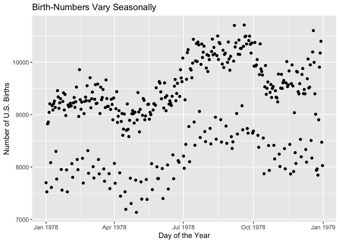
Figure 1.2: A simple scatterplot with R’s ggplot2 graphics system.
Clearly the number of births varies seasonally: more babies are born in late summer and early fall, whereas spring births are not as frequent. But there is something mysterious about the plot: Why do there are appear to be two clearly separated groups of days, one with considerably more births than the other? What is going on here? As we learn to program in R, we will gradually acquire the skills needed to answer this and many other intriguing questions.
The plot is made with the ggplot2 graphics package (Wickham et al. 2020). Graphing will not be a major focus of the course at first, but we will return from time to time, to the subject of graphing in ggplot2 as our need for graphs dictates.↩︎