4 Flow-Control

Figure 4.1: Foxtrot, October 3, 2003. Used with permission.

In the above scene from the comic-strip Foxtrot, young Jason has attempted to short-cut his “write-on-the-blackboard” punishment via some code in the C-language that would print out his assigned sentence 500 times. This is an example of flow control.

Flow control encompasses the tools in a programming language that allow the computer to make decisions and to repeat tasks. In this Chapter we will learn how flow control is implemented in R.

4.1 Prompting the User: `readline()`

One way to control the flow of a program is to arrange for it to pause and await information from the user who runs it.

Up to this point any information that we have wanted to process has had to be entered into the code itself. For example, if we want to print out a name to the console, we have to provide that name in the code, like this:

person <- "Dorothy"
cat("Hello, ", person, "!\n", sep = "")

## Hello, Dorothy!

We can get any printout we like as long as we assign the desired string to person—but we have to do that in the code itself. But what if we don’t know the name of the person whom we want to greet? How can we be assured of printing out the correct name?

The readline() function will be helpful, here. It reads input directly from the console and produces a character vector (of length one) that we may use as we like. Thus

person <- readline(prompt = "What is your name?  ")
# Type your name before running the next line!
cat("Hello, ", person, "!\n", sep = "")

## What is your name?  Cowardly Lion
## Hello, Cowardly Lion!

Note that the input obtained from readline() is always a character vector of length one—a single string—so if you plan to use it as a number then you need to convert it to a number. The as.numeric() function will do this for you:

number <- readline("Give me a number, and I'll add 10 to it:  ")
# Give R your number before you run the next line!
cat("The sum is:  ", as.numeric(number) + 10)

## Give me a number, and I'll add 10 to it:  15
## The sum is:  25

4.1.1 Practice Exercises

Try out the following code:
```
pet <- readline("Enter the name of your pet: ")
type <- readline("What kind of animal is it? (Dog, cat, etc.): ")
cat(pet, " is a ", type, ".\n", sep = "")
```
Important: Run the lines one at a time, not all three at once. R will stop after the first line, waiting for your answer. If you try to run line 2 along with the pet line, then line 2 will become your attempted input for pet, resulting in an error.

4.1.2 Solutions to the Practice Exercises

Here’s one possible outcome in the Console:

> pet <- readline("Enter the name of your pet: ")
Enter the name of your pet: Bo
> type <- readline("What kind of animal is it? (Dog, cat, etc.): ")
What kind of animal is it? (Dog, cat, etc.): dog
> cat(pet, " is a ", type, ".\n", sep = "")
Bo is a dog.

4.2 Making Decisions: Conditionals

Another type of flow control involves determining which parts of the program to execute, depending upon certain conditions.

4.2.1 `if`-Statements

Let’s design a simple guessing-game for the user:

The computer will pick randomly a whole number between 1 and 4.
The user will then be asked to guess the number.
If the user is correct, then the computer will congratulate the user.

number <- sample(1:4, size = 1)
guess <- as.numeric(readline("Guess the number (1-4):  "))
if ( guess == number ) {
  cat("Congratulations!  You are correct.")
}

The sample() function randomly picks a value from the vector that is given. The size parameter specifies how many numbers to pick. (This time we only want one number.)

Flow control enters the picture with the reserved word if. Immediately after if is a Boolean expression enclosed in parentheses. This expression is often called the condition. If the condition evaluates to TRUE, then the body of the if statement—the code enclosed in the brackets—will be executed. On the other hand if the condition evaluates to FALSE, then R skips past the bracketed code.¹³

The general form of an if expression is as follows:

if ( condition ) {
  ## code to run when the condition evaluates to TRUE
}

4.2.2 `if ... else` (and Absolute Value `abs()`)

The code above congratulates the a lucky guesser, but it has nothing at all to say to someone who did not guess correctly. The way to provide an alternative is through the addition of the else reserved-word:

number <- sample(1:4, size = 1)
guess <- as.numeric(readline("Guess the number (1-4):  "))
if ( guess == number ) {
  cat("Congratulations!  You are correct.")
} else {
  cat("Sorry, the correct number was ", number, ".\n", sep = "")
  cat("Better luck next time!")
}

The general form of an if ... else expression is as follows:

if ( condition ) {
  # code to run if the condition evaluates to TRUE
} else {
  # code to run if condition evaluates to FALSE
}

So with if ... else we can care of two alternative responses: right and wrong. But what if we want three alternatives, like this:

user guesses right;
the guess is wrong, but close to correct;
the guess isn’t even close.

First we would have to decide what it means for a guess to be “close”. In this game, let’s say that the guess is close if differs from the secret number by no more than one unit.

Next, we would have to devise a way to express “differing by no more than one unit” in R.

One way to express it is with the Boolean expression:

(guess <= number + 1) & (guess >= number - 1)

In almost-English this is:

(guess is no more than number + 1) AND (guess is at least number + 1 )

We could also focus directly on the difference: guess - number, and say that the difference needs to be between -1 and 1. In R, this is captured by the Boolean expression:

(guess - number >= -1) & (guess - number <= 1)

Yet another approach is to use the mathematical concept of absolute value. You may recall from a school math class that the absolute value of a number \(x\) is defined to be the number \(x\) itself if \(x \ge 0\), whereas it is the opposite of \(x\) if \(x < 0\). In math we write is as \(\vert x \vert\). Thus:

\(\vert 3 \vert\) is 3;
\(\vert -3 \vert\) is -(-3), which is 3;
\(\vert -5.7 \vert\) is -(-5.7), which is 5.7
\(\vert 0 \vert\) is 0.

You can say how far apart two numbers are taking the absolute value of their difference. For example,

2 and 7 are five units apart, and sure enough \(\vert 2 - 7\vert = 5\).
5 and 4 are one unit apart, and sure enough \(\vert 5 - 4\vert = 1\).

Absolute value is important enough that R has a function for it: abs(). Here is is in action:

abs(-5.7)

## [1] 5.7

abs(2 - 7)

## [1] 5

abs(5 - 4)

## [1] 1

So we can express “being close” compactly as follows:

abs(guess - number) <= 1

Now, back to the three alternatives: how do we handle them in R? Here is one way:

number <- sample(1:4, size = 1)
guess <- as.numeric(readline("Guess the number (1-4):  "))
if ( guess == number ) {
  cat("Congratulations!  You are correct.")
} else if ( abs(guess - number) <= 1 ){
  cat("You were close!\n")
  cat("The correct number was ", number, ".\n", sep = "")
} else {
  cat("You were way off.\n")
  cat("The correct number was ", number, ".\n", sep = "")
}

We chained two if ... else expressions together, so that the second if ... else is what gets evaluated if the condition in the first if ... else statement (guess == number) was FALSE.

An if ... else chain can be as long as you like. In general, a chain looks like this:

if ( condition1) {
  # code to run if condition1 evaluates to TRUE
} else if ( condition2 ) {
  # code to run if condition2 evaluates to TRUE
} else if ( condition3 ) {
  # code to run if condition2 evaluates to TRUE
} else if ......

  # and so on until
} else if ( conditionN ) {
  # code to run if conditionN evaluates to TRUE
}

4.2.3 The `ifelse()` Function

The ifelse() function is not officially flow control—it is just a function that you call like other functions—but it can get do the some of the work of an if ... else statement. Watch this:

person <- "Dorothy"
ifelse(
  test = person == "Dorothy",
  yes = "That's Dorothy, all right!",
  no = "That's someone else."
)

## [1] "That's Dorothy, all right!"

person <- "Scarecrow"
ifelse(
  test = person == "Dorothy",
  yes = "That's Dorothy, all right!",
  no = "That's someone else."
)

## [1] "That's someone else."

As you can see, ifelse() takes three parameters:

test: a Boolean expression;
yes: the result when test evaluates to TRUE
no: the result when test evaluates to FALSE

Most people don’t name the parameters when they call ifelse(), they just make sure that the arguments are in the right order, like this:

person <- "Scarecrow"
ifelse(
  person == "Dorothy", 
  "That's Dorothy, all right!", 
  "That's someone else."
)

## [1] "That's someone else."

The arguments to yes and no will be recycled to match the length of the Boolean expression test, so you can actually make many decisions at once:

person <- c("Dorothy", "Scarecrow", "Toto", "Dorothy")
ifelse(
  person == "Dorothy", 
  "That's Dorothy, all right!", 
  "That's someone else."
)

## [1] "That's Dorothy, all right!" "That's someone else."      
## [3] "That's someone else."       "That's Dorothy, all right!"

Suppose that you have a lot of heights:

height <- c(69, 67, 70, 72, 65, 63, 75, 70)

You would like to classify each person as either “tall” or “short”, depending on whether they are respectively more or less than 71 inches in height. ifelse() makes quick work of it:

heightClass <- ifelse(height > 70, "tall", "short")
heightClass

## [1] "short" "short" "short" "tall"  "short" "short" "tall"  "short"

4.2.4 An Application of `ifelse()`: Triangle Testing

Here’s another example of the power of ifelse().

If a triangle has three sides of length \(x\), \(y\) and \(z\), then the sum of any two sides must be greater than the remaining side:

\[\begin{aligned} x + y &> z, \\ x + z &> y, \\ y + z &> x. \end{aligned}\] This fact is known as the Triangle Inequality. It works the other way around, too: if three positive numbers are such that the sum of any two exceeds the third, then three line segments having those numbers as lengths could be arranged into a triangle.

We can write a function that, when given three lengths, determines whether or not they can make a triangle:

isTriangle <- function(x, y, z) {
  (x + y > z) & (x + z > y) & (y + z > x)
}

isTriangle() simply evaluates a Boolean expression involving x, y and z. It will return TRUE when the three quantities satisfy the Triangle Inequality; otherwise, it returns FALSE. Let’s try it out:

isTriangle(x = 3, y = 4, z = 5)

## [1] TRUE

Now suppose that we are would like to know which of the following six triples of numbers could be the side-lengths of a triangle:

\[(2,4,5),(4.7,1,3.8),(5.2,8,12),\\ (6, 6, 13), (6, 6, 11), (9, 3.5, 6.2)\]

We could enter the triples one at a time into isTriangle(). Here are the first two:

isTriangle(x = 2, y = 4, z = 5)     ## test first triple

## [1] TRUE

isTriangle(x = 4.7, y = 1, z = 3.8) ## test second triple

## [1] TRUE

But in the Boolean expression:

(x + y > z) & (x + z > y) & (y + z > x)

there is nothing stopping x, y and z from being vectors of length more than 1. Taking advantage of this fact, we could arrange the sides of the six triples into three vectors of length six each:

a <- c(2, 4.7, 5.2, 6, 6, 9)
b <- c(4, 1, 2.8, 6, 6, 3.5)
c <- c(5, 3.8, 12, 13, 11, 6.2)

The first elements of a, b and c are the sides of the first triple, the second elements are the sides of the second triple, and so on.

Now we can decide about all six triples at once:

isTriangle(x = a, y = b, z = c)

## [1]  TRUE  TRUE FALSE FALSE  TRUE  TRUE

Finally, we bring in ifelse() to create a new character-vector that expresses our results verbally:

triangle <- ifelse(isTriangle(a, b, c), "triangle", "not")
triangle

## [1] "triangle" "triangle" "not"      "not"      "triangle" "triangle"

4.2.5 Practice Exercises

Write a function called findKarl() that takes a character vector and returns a character vector that reports whether or not each element of the given vector was equal to the string "Karl". It should work like this:
```
vec1 <- c("three", "blowfish", "Karl", "Grindel")
findKarl(vec1)
```
```
## [1] "Sorry, not our guy." "Sorry, not our guy." "Yep, that's Karl!"  
## [4] "Sorry, not our guy."
```

Here’s a function that is supposed to return "small!" when given a number less than 100, and return "big!" when the number if at least 100:

sizeComment <- function(x) {
  if ( x < 100 ) {
    "small!"
  }
  "big!"
}

But it doesn’t work:

sizeComment(200)  # this will be OK

## [1] "big!"

sizeComment(50)   # this won't be OK

## [1] "big!"

Fix the code.

4.2.6 Solutions to Practice Exercises

Here’s one way to write it:

findKarl <- function(x) {
  ifelse(x == "Karl",
         "Yep, that's Karl!",
         "Sorry, not our guy.")
}

A function always returns the value of the last expression that it evaluates. As it stands, the function will always end at the line "big!", so "big" will always be returned. One way to get the desired behavior is to force the function to stop executing once it prints out "small!". You can do this with the return() function:
```
sizeComment <- function(x) {
  if ( x < 100 ) {
    return("small!")
  }
  "big!"
}
```
Another way is to use the if ... else construction:
```
sizeComment <- function(x) {
  if ( x < 100 ) {
    "small!"
  } else {
    "big!"
  }
}
```

4.3 Repeating Things: Looping

So far we have looked into the aspects of flow-control that pertain to:

pausing the flow of evaluation of expressions to get input from the user (readline());
deciding which expressions to evaluate, based on conditions (if and if ... else).

Let us now turn to the R-constructs that make the computer return to a body of expressions, evaluating them repeatedly. This is called looping.

4.3.1 For Loops

The reserved word for is used to make R repeat an action a specified number of times.

We begin with an very simple example:

for (i in 1:4) {
  cat("Hello, Dorothy!\n")
}

## Hello, Dorothy!
## Hello, Dorothy!
## Hello, Dorothy!
## Hello, Dorothy!

Here’s how the loop works. Recall that the vector 1:4 is simply the sequence of integers from 1 to 4:

1:4

## [1] 1 2 3 4

When R sees the code (i in 1:4) it knows that it will have to go four times through the body of the loop, which is expression in the brackets:

cat("Hello, Dorothy!\n")

At the start of the loop, the index variable i is set to 1. After the body is executed the first time, R sets i to 2, then executes the body again. Then R sets i to 3 and executes the body yet again. Then R sets i to 4, and executes the body for the final time. Four this example, the result is four lines printed out to the console.

The more you need to repeat a particular pattern, the more it makes sense to write your code with a loop.

The general form of a loop is:

for (var in seq) {
  # code that could involve var
}

var is the index variable, and it can be any permitted name for a variable, and seq can be any vector. As R traverses the loop, the value of the index variable var becomes each element of the vector seq in turn. With every change in the value of var, the code in the brackets is executed.

In general, the expressions that make up the body of the loop could make reference to the index var. In our example above, the body did not do this, as the purpose of the iteration was just to execute the body four times.

To iterate is to do a thing again and again. The vector seq is sometimes called an iterable, since it is “iterated over.” It contains the values that the index variable will assume, one by one, as the loop is repeated.

It’s important to realize that the index variable can have any valid name, and the sequence can be any type of vector at all—not just a sequence of consecutive whole numbers beginning with 1. This level of generality permits a for-loop to automate a wide variety of tasks, and for its code to be written in a way that evokes the operations being performed.

For example, here is a loop to print out some greetings;

people <- c("Dorothy", "Tin Man", "Scarecrow", "Lion")
for (person in people) {
  cat("Hello, ", person, "!\n", sep = "")
}

## Hello, Dorothy!
## Hello, Tin Man!
## Hello, Scarecrow!
## Hello, Lion!

Note that in this example, the body DOES make reference to the index person, so R gives a different result each time it goes through the loop.

Maybe you want to report on the squares of the first ten natural numbers. One way to do it is:

for (i in 1:10) {
  cat("The square of ", i, " is ", i^2, ".\n", sep = "")
}

## The square of 1 is 1.
## The square of 2 is 4.
## The square of 3 is 9.
## The square of 4 is 16.
## The square of 5 is 25.
## The square of 6 is 36.
## The square of 7 is 49.
## The square of 8 is 64.
## The square of 9 is 81.
## The square of 10 is 100.

Here is another way:

numbers <- 1:10
for (number in numbers) {
  cat(
    "The square of ", number, " is ", 
    number^2, ".\n", sep = ""
  )
}

## The square of 1 is 1.
## The square of 2 is 4.
## The square of 3 is 9.
## The square of 4 is 16.
## The square of 5 is 25.
## The square of 6 is 36.
## The square of 7 is 49.
## The square of 8 is 64.
## The square of 9 is 81.
## The square of 10 is 100.

4.3.1.1 Iterating “By Index”

Think back to the loop we wrote to greet people:

people <- c("Dorothy", "Tin Man", "Scarecrow", "Lion")
for (person in people) {
  cat("Hello, ", person, "!\n", sep = "")
}

In this loop, the iterable people contains all of the values that we need to work with in the body of the loop. But what if we had to access information contained in two or more vectors?

For example, we might have the following information on some people:

people <- c("Dorothy", "Tin Man", "Scarecrow", "Lion")
heights <- c(62, 72, 70, 75)
desires <- c("Kansas", "brains", "a heart", "courage")

We would like to greet each person in turn, stating their age and desire as we do so.

In this case it would not be convenient to use any of the above three vectors as the iterable in a for-loop. Instead, it is better to use a vector of the indices of the three vectors—the numbers 1, 2, 3 and 4—as our iterable:

for (i in 1:length(people)) {
  cat(
    "Hello, ", people[i], "!\n", 
    " You are ", heights[i], " inches tall.\n",
    "Your desire is:  ", desires[i], ".\n\n",
    sep = "")
}

## Hello, Dorothy!
##  You are 62 inches tall.
## Your desire is:  Kansas.
## 
## Hello, Tin Man!
##  You are 72 inches tall.
## Your desire is:  brains.
## 
## Hello, Scarecrow!
##  You are 70 inches tall.
## Your desire is:  a heart.
## 
## Hello, Lion!
##  You are 75 inches tall.
## Your desire is:  courage.

When we get at the values we want by way of their indices in a vector, using the indices themselves as our iterable, then we are said to be iterating by index.

4.3.1.2 Using a Loop to Store Results

Quite often you will want to store the results of your trips through the loop. Let’s do this for squaring numbers:

squares <- numeric(length = 10)

We used the numeric() function to create the type-double vector squares. We specified that the number of elements in squares shall be the same as the number of numbers that we want to square.

Right now squares isn’t very interesting, as all of its elements are 0:

squares

##  [1] 0 0 0 0 0 0 0 0 0 0

It is just a placeholder for the squares that are to come.

We will now write a for-loop to fill squares with the desired squares:

for (i in 1:length(squares)) {
  squares[i] <- i^2
}

(Note that the iterable was 1:10, because squares was set up to be of length 10.)

Now each of the four elements of squares contains the square of the corresponding element of 1:10:

squares

##  [1]   1   4   9  16  25  36  49  64  81 100

Let’s try another, more whimsical application. This example involves colors.

R has a function called color() that, when called, returns a vector of all the colors that R is prepared to recognize by name. To see them all, run the following for yourself:

colors()

Here are the first ten of them:

colors()[1:10]

##  [1] "white"         "aliceblue"     "antiquewhite"  "antiquewhite1"
##  [5] "antiquewhite2" "antiquewhite3" "antiquewhite4" "aquamarine"   
##  [9] "aquamarine1"   "aquamarine2"

R has another function called sample(), that will pick elements at random from a vector. We will learn more about it in the following chapter. For now, let’s just use it to pick one color ar random:

sample(colors(), size = 1)

## [1] "grey13"

Try it for yourself, to see that you get different colors each time you run the code.

Now imagine that Scarecrow is walking through a meadow filled with flowers. Ten times he stoops to pick up a flower. We want to keep a record of the colors that he got each time. Here is how we might do it:

reports <- character(length = 10)

We used the character() function to create a place-holder vector to hold the our results. Right now it is just a vector of empty strings:

reports

##  [1] "" "" "" "" "" "" "" "" "" ""

We can use a loop to fill it up:

for (i in 1:length(reports)) {
  color <- sample(colors(), size = 1)
  outcome <-  paste(
    "Flower ", i, 
    " is ", color, ".", sep = ""
  )
  reports[i] <- outcome
}

Now we have our record of what happened:

reports

##  [1] "Flower 1 is yellow2."        "Flower 2 is grey7."         
##  [3] "Flower 3 is gray48."         "Flower 4 is mistyrose1."    
##  [5] "Flower 5 is moccasin."       "Flower 6 is darkgoldenrod3."
##  [7] "Flower 7 is lightslateblue." "Flower 8 is antiquewhite2." 
##  [9] "Flower 9 is grey64."         "Flower 10 is bisque1."

Note that the name of the index variable does not matter. We could have got the same results with:

for (flower_number in 1:length(reports)) {
  color <- sample(colors(), size = 1)
  outcome <-  paste(
    "Flower ", flower_number, 
    " is ", color, ".", sep = ""
  )
  reports[flower_number] <- outcome
}

Usually, though, when the index variable refers to the index of some vector, we use a short name like i or j that prompts the reader to think: “Oh, this is a number that varies as we go through the loop.”

You will often have reason to set up a placeholder vector of a definite length and use a loop to store information in it. The general format is this:

# make placeholder vector:
results <- numeric/character/logical(someLength) 

# fill it up:
for ( i in 1:someLength ) {
  # computations involving i, and then:
  results[i] <- some_result_depending_on_i
}

# later on do things with results, such as:
print(results)

As you see, the results vector could also be constructed with logical() if you plan to store TRUEs and FALSEs.

4.3.2 Breaking Out of a Loop

Sometimes you finish the task at hand before you are done with the loop. If this is a possibility for you then you may arrange to break out of the loop with the break reserved-word.

Suppose for example that you want a function that searches through a vector for a given element, updating the user along the way as to the progress of the search. You can try something like this:

# function to find index of element in vector.
# returns -1 if elem is not in vector
verboseSearch <- function(elem, vec) {
  
  # The following logical keeps track of whether
  # we have found the element.
  # We have not yet begun the search so start it
  # at FALSE.
  found <- FALSE
  
  # check the elements of vector:
  for ( i in 1: length(vec) ) {
    if ( vec[i] == elem ) {
      # record that we found the element:
      found <- TRUE
      break
    } else {
      # report no match at this index:
      cat("Checked index ", i, 
          " in the vector.  No match there ...\n", sep = "")
    }
  }
  
  if ( found ) {
    # report success:
    cat("Found ", elem, " at index ", i, ".\n", sep = "")
    return(i)
  } else {
    # report failure:
    cat(elem, " is not in the vector.\n", sep = "")
    return(-1)
  }
}

Let’s see our function in action:

people <- c("Dorothy", "Tin Man", "Scarecrow", "Lion")
scarecrowPlace <- verboseSearch("Scarecrow", people)

## Checked index 1 in the vector.  No match there ...
## Checked index 2 in the vector.  No match there ...
## Found Scarecrow at index 3.

4.3.3 `while`-Loops

For-loops are pretty wonderful, but they are best used in circumstances when you know how many times you will need to loop. When you need to repeat a block of code until a certain condition occurs, then the while reserved-word might be a good choice.

A while-loop runs as long as a specified condition is true. The general format is this:

while (Boolean_condition) {
  ## code to run goes here
}

The condition evaluated prior to the body of the loop. If the condition evaluates to TRUE, then R does not evaluate the the code in the body of the loop. If it is TRUE, then R evaluates the body, and then checks the condition again. R will repeatedly evaluate the body of the loop until the condition evaluates to FALSE, at which point R moves on to whatever code comes after the loop.

4.3.3.1 Application: In a Meadow, Picking Flowers

Suppose, for example, that Scarecrow is walking through a field that contains flowers of the following colors:

flower_colors <- c("blue", "pink", "crimson")

Let’s have Scarecrow walk through the field and pick flowers until he gets two blue flowers. We would like a report of his activities.

We begin by setting up a vector for the results:

reports <- character()

The default value for length is 0, so at the moment this is an empty character vector:

reports

## character(0)

We did this because we don’t know how many flowers Scarecrow will pick before getting his second blue flower. Our plan is to fill it up with reports for each flower picked.

We will use a while-loop:

count <- 0
i <- 1
while (count < 2) {
  flower <- sample(flower_colors, size = 1)
  outcome <- paste(
    "On pick ", i, ", Scarecrow got a ",
    flower, " flower.", sep = ""
  )
  reports[i] <- outcome
  i <- i + 1
  if (flower == "blue") count <- count + 1
}

Let’s see what happened:

reports

##  [1] "On pick 1, Scarecrow got a crimson flower." 
##  [2] "On pick 2, Scarecrow got a pink flower."    
##  [3] "On pick 3, Scarecrow got a pink flower."    
##  [4] "On pick 4, Scarecrow got a pink flower."    
##  [5] "On pick 5, Scarecrow got a crimson flower." 
##  [6] "On pick 6, Scarecrow got a pink flower."    
##  [7] "On pick 7, Scarecrow got a pink flower."    
##  [8] "On pick 8, Scarecrow got a crimson flower." 
##  [9] "On pick 9, Scarecrow got a pink flower."    
## [10] "On pick 10, Scarecrow got a pink flower."   
## [11] "On pick 11, Scarecrow got a blue flower."   
## [12] "On pick 12, Scarecrow got a crimson flower."
## [13] "On pick 13, Scarecrow got a crimson flower."
## [14] "On pick 14, Scarecrow got a blue flower."

If you try it, your results will likely be different!

It would be fun to encapsulate our work into a function:

scarecrow_walk <- function(flower_colors, blues_desired) {
  reports <- character()
  count <- 0
  i <- 1
  while (count < blues_desired) {
    flower <- sample(flower_colors, size = 1)
    outcome <- paste(
      "On pick ", i, ", Scarecrow got a ",
      flower, " flower.", sep = ""
    )
    reports[i] <- outcome
    i <- i + 1
    if (flower == "blue") count <- count + 1
  }
  reports
}

Let’s try it:

pick_record <- scarecrow_walk(
  flower_colors = c("red", "pink", "burlywood", "blue"),
  blues_desired = 5
)

How many flowers did Scarecrow pick? This many:

picks <- length(pick_record)
picks

## [1] 19

Here is a record of the final five picks:

pick_record[(picks - 4):picks]

## [1] "On pick 15, Scarecrow got a burlywood flower."
## [2] "On pick 16, Scarecrow got a burlywood flower."
## [3] "On pick 17, Scarecrow got a red flower."      
## [4] "On pick 18, Scarecrow got a pink flower."     
## [5] "On pick 19, Scarecrow got a blue flower."

When you use a while-loop, you be very careful to program it so that eventually the Boolean condition becomes FALSE. Otherwise, R will repeat the loop forever. This is called an infinite loop.

For example, suppose that the user were make the following call:

scarecrow_walk(
  flower_colors = c("red", "pink", "burlywood"),
  blues_desired = 5
)

Scarecrow would never pick a blue flower, so count < blues_desired would never become FALSE. This is a big enough problem that we should modify the function to reject any field that does not have blue flowers:

scarecrow_walk <- function(flower_colors, blues_desired) {
  if (!("blue" %in% flower_colors)) {
    return(cat("Your field needs blue flowers."))
  }
  reports <- character()
  count <- 0
  i <- 1
  while (count < blues_desired) {
    flower <- sample(flower_colors, size = 1)
    outcome <- paste(
      "On pick ", i, ", Scarecrow got a ",
      flower, " flower.", sep = ""
    )
    reports[i] <- outcome
    i <- i + 1
    if (flower == "blue") count <- count + 1
  }
  reports
}

Now the infinite loop is warded off:

scarecrow_walk(
  flower_colors = c("red", "pink", "burlywood"),
  blues_desired = 5
)

## Your field needs blue flowers.

4.3.3.2 Application: A Better Guessing Game

Earlier when studied the conditionals if and if ... else (Section 4.2), we worked on a game where the user was invited to guess a secret number. It wasn’t very fun because the user only got to guess once.

With while-loops in hand, we can return to the game and make it much more interesting.

n <- 20
number <- sample(1:n, size = 1)
cat("I'm thinking of a whole number from 1 to ", n, ".\n", sep = "")
guessing <- TRUE
while (guessing) {
  guess <- readline("What's your guess? (Enter q to quit.)  ")
  if ( guess == "q"  ) {
    cat("Bye!\n")
    break
  } else if ( as.numeric(guess) == number ) {
    guessing <- FALSE
    cat("You are correct!  Thanks for playing!")
  }
  # If we get here, the guess was not correct:
  # loop will repeat!
}

Of course, if the user is playing the game in RStudio, the secret number shows up in the Global Environment. We can make the game more realistic by encapsulating it into a function:

guess_my_number <- function(n) {
  number <- sample(1:n, size = 1)
  cat("I'm thinking of a whole number from 1 to ", n, ".\n", sep = "")
  guessing <- TRUE
  while (guessing) {
    guess <- readline("What's your guess? (Enter q to quit.)  ")
    if ( guess == "q"  ) {
      cat("Bye!\n")
      break
    } else if ( as.numeric(guess) == number ) {
      guessing <- FALSE
      cat("You are correct!  Thanks for playing!")
    }
  }
}

The game works well enough, but if you give it a try, you are sure to find it a bit fatiguing when n is set to a large value—it would be kind to give the user a hint after an incorrect guess. Let’s revise the function to tell the reader whether her guess was high or low:

guess_my_number_improved <- function(n) {
  number <- sample(1:n, size = 1)
  cat("I'm thinking of a whole number from 1 to ", n, ".\n", sep = "")
  guessing <- TRUE
  while (guessing) {
    guess <- readline("What's your guess? (Enter q to quit.)  ")
    guessing <- TRUE
    if (guess == "q") {
      cat("Bye!\n")
      break
    } else if (as.numeric(guess) == number) {
      guessing <- FALSE
      cat("You are correct!  Thanks for playing!")
    } else {
       # If we get to this point the guess was not correct.
      # Issue hint:
      hint <- ifelse(as.numeric(guess) > number, "high", "low")
      cat("Your guess was ", hint, ".  Keep at it!\n", sep = "")
    }
    # if still guessing, we will repeat the loop
  }
}

There is no limit to the complexity of games you can create with functions and various combinations of the flow-control tools in this Chapter.

4.3.4 Practice Exercises

You want to compute the square roots of the whole numbers from 1 to 10. You could do this quite easily as follows:
```
sqrt(1:10)
```
```
##  [1] 1.000000 1.414214 1.732051 2.000000 2.236068 2.449490 2.645751
##  [8] 2.828427 3.000000 3.162278
```
However, you want to practice using for-loops. Write a small program that uses a loop to compute the square roots of the whole numbers from 1 to 10.
Think about the practice problem findKarl() from the previous section. Write a new version that uses a loop.
You want to append "the Dog" to the end of each element of a character vector of dog-names. Sadly, you have not yet realized that the paste() function is very much up to the task:
```
doggies <- c("Bo", "Gracie", "Rover", "Anya")
paste(doggies, "the Dog")
```
```
## [1] "Bo the Dog"     "Gracie the Dog" "Rover the Dog" 
## [4] "Anya the Dog"
```
You decide to use a for-loop. Write the code.
Write a function called triangleOfStars() that produces patterns like this:
```
****
***
**
*
```
It should take a single parameter n, the number of asterisks in the first “line” of the triangle. Use a for-loop in the body of the function.
Write a function called trianglePattern() that produces patterns like the ones from the previous problem, but using any character that the user specifies. The function should take two parameters:
- char, a string giving the character to use. The default value should be "*".
- n, the number of asterisks in the first “line” of the output.
Typical examples of use should be as follows:
```
trianglePattern(char = "x", 5)
```
```
## xxxxx
## xxxx
## xxx
## xx
## x
```
```
trianglePattern(n = 6)
```
```
## ******
## *****
## ****
## ***
## **
## *
```
Rewrite triangleOfStars() so that it uses a while-loop in its body.
Rewrite triangleOfStars() so that it still uses a while-loop in its body, but produces output like this:
```
*
**
***
****
```
Write a function called ageReporter() that reports the ages of given individuals. It should take two parameters:
- people: a character vector of names of the people of interest.
- ages: a vector containing the ages of the people of interest.
The two vectors should be of the same length.

Typical examples of use would be as follows:
```
folks <- c("Gina", "Hector")
theirAges <- c(25, 22)
ageReporter(folks, theirAges)
```
```
## Gina is 25 year(s) old.
## Hector is 22 year(s) old.
```

4.3.5 Solutions to the Practice Exercises

Here’s a suitable program:

roots <- numeric(10)
for ( i in 1:10 ) {
  roots[i] <- sqrt(i)
}
roots

##  [1] 1.000000 1.414214 1.732051 2.000000 2.236068 2.449490 2.645751
##  [8] 2.828427 3.000000 3.162278

You could do this:

findKarl <- function(x) {
  results <- character(length(x))
  for ( i in 1: length(x) ) {
    if ( x[i] == "Karl" ) {
      results[i] <- "Yep, that's Karl!"
    } else {
      results[i] <-  "Sorry, not our guy."
    }
  }
  results
}

Here you go:

doggies <- c("Bo", "Gracie", "Rover", "Anya")
titledDoggies <- character(length(doggies))
for (i in 1:length(doggies) ) {
  titledDoggies[i] <- paste(doggies[i], "the Dog")
}
titledDoggies

## [1] "Bo the Dog"     "Gracie the Dog" "Rover the Dog" 
## [4] "Anya the Dog"

Here’s the code:

triangleOfStars <- function(n) {
  for ( i in n:1 ) {
    line <- rep("*", times = i)
    cat(line, "\n", sep = "")
  }
}

Try it out:

triangleOfStars(5)

## *****
## ****
## ***
## **
## *

Here’s the code:

trianglePattern <- function(char = "*", n) {
  for (i in n:1) {
    line <- rep(char, times = i)
    cat(line, "\n", sep = "")
  }
}

Here’s the code:

triangleOfStars <- function(n) {
  while ( n >= 1 ) {
    line <- rep("*", times = n)
    cat(line, "\n", sep = "")
    n <- n - 1
  }
}

Try it out:

triangleOfStars(5)

## *****
## ****
## ***
## **
## *

Here’s the code:

triangleOfStars <- function(n) {
  m <- 1
  while ( m <= n ) {
    line <- rep("*", times = m)
    cat(line, "\n", sep = "")
    m <- m + 1
  }
}

Try it out:

triangleOfStars(5)

## *
## **
## ***
## ****
## *****

We can solve this problem easily if we iterate by index:

ageReporter <- function(people, ages) {
  for (i in 1:length(people)) {
    cat(people[i], " is ", ages[i], " year(s) old.\n", sep = "")
  }
}

4.4 Nested Loops

Suppose that as they walk along the Yellow Brick Road, our Oz friends come upon a meadow that has flowers of the following colors:

flower_colors <- c("blue", "red", "pink", "crimson", "orange")

The friends decide to wander through this meadow, looking for a certain number of their favorite flowers:

Dorothy likes blue flowers, and wants 3 of them.
Tin Man likes red flowers, and wants 2 of them.
Scarecrow like blue flowers, and wants 2 of them.
Lion likes crimson flowers, and wants 5 of them.
Toto likes pink flowers, and wants 1 of them.

We record this information as follows:

friends <- c("Dorothy", "Tin Man", "Scarecrow", "Lion", "Toto")
fav_color <- c("blue", "red", "blue", "crimson", "pink")
number_wanted <- c(3, 2, 2, 5, 1)

We would like to write a function that makes each person take turns wandering through the field until he/she has collected the desired number of his/her desired flowers. We want the function to return the total number of flowers collected by everyone. Along the way, the function should report what flowers each person collects.

An outline for the code in the body of the function would be:

for (person in people) {
  while (person_is_picking_flowers) {
    ## report on flowers picked
    ## somehow keep track of how many are picked
  }
  ## return the total flowers picked
}

This is a loop within a loop: nested loops, they are called.

Writing nested loops can be quite difficult. It is probably a good idea to simplify the problem, at first, by writing a function that does the required work for just one person.

Below is such a function. It takes three parameters:

person: the name of the person walking through the meadow;
color: the color of the flower the person is looking for;
wanted: how many flowers of the desired color the person wants.
report: whether or not to report what flowers are picked. The default value is FALSE.

The function will optionally report the flowers collected as a side-effect, and will return the number of flowers collected:

walk_meadow <- function(person, color, wanted, report = FALSE) {
  picking <- TRUE
  pick_count <- 0
  desired_count <- 0
  if (report) {
    cat(person, " picks flowers of the following colors: ")
  }
  while (picking) {
    picked <- sample(flower_colors, size = 1)
    pick_count <- pick_count + 1
    if (picked == color) desired_count <- desired_count + 1
    if (desired_count == wanted) picking <- FALSE
    if (report) {
      message <- ifelse(
        picking,
        paste(picked, ", ", sep = ""),
        paste(picked, ".\n\n", sep = "")
      )
      cat(message)
    }
  }
  pick_count
}

Let’s try it on another person, the Quadling Boq:

walk_meadow(
  person = "Boq",
  color = "blue",
  wanted = 3,
  report = TRUE
)

## Boq  picks flowers of the following colors: crimson, crimson, blue, blue, crimson, red, blue.

## [1] 7

With this helper-function in hand, it’s easier to write the desired function:

all_walk <- function(people, favs, 
                     numbers, report) {
  total <- 0
  for (i in 1:length(people)) {
    person <- people[i]
    fav <- favs[i]
    number <- numbers[i]
    flowers_picked <- walk_meadow(
      person = person,
      color = fav,
      wanted = number,
      report = report
    )
    total <- total + flowers_picked
  }
  total
}

Recall our information:

friends <- c("Dorothy", "Tin Man", "Scarecrow", "Lion", "Toto")
fav_color <- c("blue", "red", "blue", "crimson", "pink")
number_wanted <- c(3, 2, 2, 5, 1)

We try the function on this information:

all_walk(
  people = friends,
  favs = fav_color,
  numbers = number_wanted,
  report = TRUE
)

## Dorothy  picks flowers of the following colors: orange, red, red, orange, red, pink, red, orange, crimson, red, crimson, crimson, red, crimson, orange, crimson, crimson, pink, red, red, pink, orange, crimson, orange, orange, red, orange, blue, pink, orange, blue, orange, pink, blue.
## 
## Tin Man  picks flowers of the following colors: orange, pink, red, red.
## 
## Scarecrow  picks flowers of the following colors: blue, pink, red, blue.
## 
## Lion  picks flowers of the following colors: orange, orange, red, orange, crimson, pink, crimson, crimson, red, red, blue, blue, crimson, red, red, red, blue, crimson.
## 
## Toto  picks flowers of the following colors: blue, blue, crimson, red, red, orange, orange, crimson, crimson, crimson, orange, crimson, blue, orange, blue, crimson, crimson, pink.

## [1] 78

If we don’t need the reports, we just set report to FALSE:

all_walk(
  people = friends,
  favs = fav_color,
  numbers = number_wanted,
  report = FALSE
)

## [1] 71

4.4.1 Practice Exercises

Write a function called cheerleader() that badgers you for each of the letters in a word until you give it all of the letters, one by one. It should work like this:

schoolMascot <- c("T", "I", "G", "E", "R", "S")
cheerleader(cheer = schoolMascot)

> cheerleader(cheer = schoolMascot)
Gimme a T!  T
Gimme a I!  i
Gimme a I!  I
Gimme a G!  gee
Gimme a G!  I said gee!!
Gimme a G!  G
Gimme a E!  E
Gimme a R!  Are you going to do this all day?
Gimme a R!  R
Gimme a S!  Stop it, please!
Gimme a S!  S
>

Solutions to the Practice Exercises

First write a helper-function:

badger_for_item <- function(item) {
  badgering <- TRUE
  while (badgering) {
    call <- paste("Gimme a ", item, "!  ", sep = "")
    response <- readline(call)
    if ( response == item ) badgering <- FALSE
   }
}

Try it out in the console:

badger_for_item(item = "T")

Now write the required function:

cheerleader <- function(cheer) {
  for (element in cheer) {
    badger_for_item(item = element)
  }
}

If you have the patience, try it out in the console:

cheerleader(cheer = c("D", "U", "C", "K", "S"))

4.5 More in Depth

4.5.1 Validating Arguments

Recall the function manyCat():

manyCat <- function(word, n) {
  wordWithNewline <- paste(word, "\n", sep = "")
  lines <- rep(wordWithNewline, times = n)
  cat(lines, sep = "")
}

What would happen if a user were to call it with an unusable argument for the parameter n, a negative number, for instance?

manyCat(word = "Hello", n = -3)

## Error in rep(wordWithNewline, times = n): invalid 'times' argument

For us, it’s clear enough what is wrong. After all, we wrote the function in the previous chapter, and we know that the rep() function in its body requires that the times parameter be set to some positive integer. On the other hand, to someone who is unfamiliar with the body of manyCat() and who has no access to help on how manyCat() is to be used it may not be so obvious what has gone wrong and why.

In the case of complex functions, we cannot expect ordinary users to search through the function’s definition to learn how to fix an error that arises from improper input. Accordingly, it can be good practice to validate user-input. Conditionals allow us to do this.

Here, a possible approach is to attempt to coerce the user’s input for n into an integer, using the as.integer() function:

as.integer(3.6) # will round to nearest integer

## [1] 3

as.integer("4") # will convert string to number 4

## [1] 4

as.integer("4.3") # will convert AND round

## [1] 4

as.integer("two") # cannot convert to integer

## Warning: NAs introduced by coercion

## [1] NA

In the last example, the result is NA, and a cryptic warning was issued. In order to keep the warning from the user, we should wrap any call to as.integer() in the suppressWarnings() function.

Let’s try out a piece of code that checks for validity:

n <- "two"  # this will not convert to a number at all
converted <- suppressWarnings(as.integer(n))
!is.na(converted) && converted >= 1

## [1] FALSE

Think about what happened:

First we attempted to converted the "two" to an integer.
Since the result of as.integer("two") is NA, the expression is.na(converted) evaluates to TRUE
Hence !is.na(converted) evaluates to FALSE.
Hence !is.na(converted) && converted > 1 evaluates to FALSE.

Let’s try it on another “wrong” value:

n <- -2  # number, but it's negative
converted <- suppressWarnings(as.integer(n))
!is.na(converted) && converted >= 1

## [1] FALSE

This time converted gets an assigned value, namely -2, but since it’s not at least 1 the expression !is.na(converted) && converted >= 1 evaluates to FALSE.

Now let’s try it on a “good” value:

n <- 3
converted <- suppressWarnings(as.integer(n))
!is.na(converted) && converted >= 1

## [1] TRUE

Our code appears to be working well.

Now that we’ve figured out a way to determine whether any given input is a usable number, let’s employ a conditional to implement validation in manyCat():

manyCat <- function(word, n) {
  n <- suppressWarnings(as.integer(n))
  isValid <- !is.na(n) && n >= 1
  if (!isValid) {
    message <- "Sorry, n must be a whole number at least 1.\n"
    return(cat(message))
  }
  wordWithNewline <- paste(word, "\n", sep = "")
  lines <- rep(wordWithNewline, times = n)
  cat(lines, sep = "")
}

The idea is to force an early return—along with a helpful message to the Console—if the user’s argument for n is no good.

Let’s watch it in action:

manyCat(word = "Hello", n = "two")   # problem!

## Sorry, n must be a whole number at least 1.

manyCat(word = "Hello", n = 3)       # OK

## Hello
## Hello
## Hello

Validation is very commonly called-for. Recall, for instance, the verboseSearch() that we wrote earlier in this Chapter:

verboseSearch <- function(elem, vec) {
  found <- FALSE

  for (i in 1: length(vec)) {
    if (vec[i] == elem) {
      found <- TRUE
      break
    } else {
      cat("Checked index ", i, 
          " in the vector.  No match there ...\n", sep = "")
    }
  }
  
  if (found) {
    cat("Found ", elem, " at index ", i, ".\n", sep = "")
    return(i)
  } else {
    cat(elem, " is not in the vector.\n", sep = "")
    return(-1)
  }
}

What would happen if, for some reason, we asked to see whether something was in a vector of length zero? Let’s see:

verboseSearch(elem = "Toto", vec = character())

## Error in if (vec[i] == elem) {: missing value where TRUE/FALSE needed

Examining the code for the function, we see that if vec has length 0, then the iterable for the for-loop is the vector 1:0 Hence the loop begins with the index i set to 1.

Within the body of the loop, R has to check evaluate the condition for the if-statement: vec[i] == elem. Since i is 1, R needs to find the first element of vec. But this time vec has length zero, so there is no first element.

Let’s see what happens when we ask for the first element of an empty vector:

character()[1]

## [1] NA

So R must then evaluate whether that NA is equal to elem, which in this case is "Toto". The result is:

NA == "Toto"

## [1] NA

But the condition for an if-statement has to evaluate either to TRUE or to FALSE. R cannot work with an NA. Hence the error message:

Error in if (vec[i] == elem) { : missing value where TRUE/FALSE needed

Whew! That was a bit of work. Let’s re-write the function with some validation, to reject length-zero vectors:

verboseSearch <- function(elem, vec) {
  found <- FALSE
  
  # validation:
  if (length(vec == 0)) {
    return(cat("vec must have at least one element."))
  }

  for (i in 1: length(vec)) {
    if (vec[i] == elem) {
      found <- TRUE
      break
    } else {
      cat("Checked index ", i, 
          " in the vector.  No match there ...\n", sep = "")
    }
  }
  
  if (found) {
    cat("Found ", elem, " at index ", i, ".\n", sep = "")
    return(i)
  } else {
    cat(elem, " is not in the vector.\n", sep = "")
    return(-1)
  }
}

The moral of the story is:

When you write functions it can be helpful to have the function validate its input instead of allowing R to throw obscure error messages at the user.

4.5.2 Solving the Empty-Vector Problem in `for`-Loops with `seq_along()`

In the previous section we considered a possible problem with for-loops of the following form:

for (i in 1:length(vec) ) {
  ## do something ...
}

In the above loop vec could be thought of as a “loop-defining” vector: its length determines the sequence of values 1, 2, 3 … for the index i. This sequence of values is supposed to end at the length of vec.

The problem is that if vec happens to be an empty vector then we probably don’t want to enter the loop at all. However, the length of an empty vector is 0, and so the vector 1:length(vec) actually works out to be a vector with two elements:

c(1,0)

Hence R will go through the loop twice: once when i is 1, and again when i is 0. Depending on what the loop does, very unexpected results could be produced.

In the previous section we dealt with the problem by writing an if-statement that provides the proper response when vec is empty. In many circumstances however, all we need to do is to make sure that the loop is skipped when the vector is empty.

A handy way to ensure skipping is to use the function seq_along() . Given any non-empty vector, seq_along() produces a sequence-vector that begins with 1 and ends with the length of the vector, thus:

vec <- c("a", "d", "f")
seq_along(vec)

## [1] 1 2 3

On the other hand, if the vector is empty, then seq_long() returns an empty numeric vector:

vec <- character()
seq_along(vec)

## integer(0)

Now consider the loop inside the following function:

loopy <- function(vec) {
  for ( i in seq_along(vec) ) {
    cat("This time i is ", i, ".\n", sep = "")
  }
}

Given a non-empty vector, it goes through the loop a number of times equal to the length of the vector:

loopy(c("a", "d", "f"))

## This time i is 1.
## This time i is 2.
## This time i is 3.

On the other hand, when given an empty vector the function does not enter the loop at all:

loopy(character())  # no output to console!

When you are writing a program that is complex enough that you don’t know whether the loop-defining vector might be empty, it is good practice to use seq_along() as a safeguard.

4.5.3 Invisible Returns

Let’s think again about the \(\pi\)-computing function from Section 3.4:

madhavaPI <- function(n = 1000000) {
  k <- 1:n
  terms <- (-1)^(k+1)*4/(2*k-1)
  sum(terms)
}

We could use if to write in a “talky” option:

madhavaPI <- function(n = 1000000, verbose = FALSE) {
  k <- 1:n
  terms <- (-1)^(k+1)*4/(2*k-1)
  approx <- sum(terms)
  if ( verbose) {
    cat("Madhava's approximation is:  ", approx, ".\n", sep = "")
    cat("This is based on ", n, " terms.\n", sep = "")
  }
  approx
}

Try it out:

madhavaPI(n = 1000, verbose = TRUE)

## Madhava's approximation is:  3.140593.
## This is based on 1000 terms.

## [1] 3.140593

It’s a bit awkward that the approximation gets printed out at the end: after the message on the console, the user doesn’t need to see it. But if we were to remove the final approx expression, then the function would not return an approximation that could be used for further computations.

The solution to this dilemma is R’s invisible() function.

madhavaPI <- function(n = 1000000, verbose = FALSE) {
  k <- 1:n
  terms <- (-1)^(k+1)*4/(2*k-1)
  approx <- sum(terms)
  if ( verbose) {
    cat("Madhava's approximation is:  ", approx, ".\n", sep = "")
    cat("This is based on ", n, " terms.\n", sep = "")
  }
  invisible(approx)
}

If you wrap an expression in invisible(), then it won’t be printed out to the console:

madhavaPI(n = 1000, verbose = TRUE)

## Madhava's approximation is:  3.140593.
## This is based on 1000 terms.

Nevertheless it is still returned, as we can see from the following code, in which the approximation is computed without any output to the console and stored in the variable p for use later on in a cat() statement.

p <- madhavaPI() # verbose is FALSE by default
cat("Pi plus 10 is about ", p + 10, ".", sep = "")

## Pi plus 10 is about 13.14159.

4.5.4 Switch

If you have to make a decision involving two or more alternatives you can use a chain of if ... else constructions. When the alternatives involve no more than the assignment of a value to a variable, you might also consider using the switch() function.

For example, suppose that you have days of the week expressed as numbers. Maybe it’s like this:

1 stands for Sunday
2 for Monday
3 for Wednesday
and so on.

If you would like to convert a day-number to the right day name, then you could write a function like this:

dayWord <- function(dayNumber) {
  switch(dayNumber,
         "Sunday",
         "Monday",
         "Tuesday",
         "Wednesday",
         "Thursday",
         "Friday",
         "Saturday")
}
dayWord(3)

## [1] "Tuesday"

In switch() above, the first argument after dayNumber is what goes with 1, the second argument is what goes with 2, and so on.

When the item you want to convert is a string rather than a number, then the switch() function works a little bit differently. Suppose, for instance, that you want to abbreviate the names of the weekdays. You might write an abbreviation-function as follows:

abbrDay <- function(day) {
  switch(
    day,
    Monday = "Mon",
    Tuesday = "Tue",
    Wednesday = "Wed",
    Thursday = "Th",
    Friday = "Fri",
    Saturday = "Sat"
  )
}
abbrDay("Wednesday")

## [1] "Wed"

In the above call to switch(), the weekday names you want to abbreviate appear as the names of named character-vectors, each of length one. The value of each vector is what the its name will be converted to.

When you are converting strings you have the option to provide a default conversion for values that don’t fit into the pattern you have in mind. All you have to do is to provide the default value as an additional argument. (It should NOT have a name.) Thus:

abbrDay <- function(day) {
  switch(
    day,
    Monday = "Mon",
    Tuesday = "Tue",
    Wednesday = "Wed",
    Thursday = "Th",
    Friday = "Fri",
    Saturday = "Sat",
    "not a weekday!"
  )
}
abbrDay("Wednesday")

## [1] "Wed"

abbrDay("Neptune")

## [1] "not a weekday!"

4.5.5 For-Loop Caution

When you write a loop you might need to exercise some caution in your choice name for the index variable. If you are already using it as the name for a variable in the same environment, then you will overwrite that variable, as demonstrated by the following code:

day <- "Thursday"
cat("Today is ", day, ".\n", sep = "")

## Today is Thursday.

weekdays <- c("Saturday", "Monday", "Friday", "Saturday")
abbrDays <- character(length(weekdays))
for ( day in weekdays ) {
  print(day)
}

## [1] "Saturday"
## [1] "Monday"
## [1] "Friday"
## [1] "Saturday"

cat("Today is ", day, ".\n", sep = "")

## Today is Saturday.

Of course, that won’t happen if the for-loop is inside of a function and your variable is outside of it.

day <- "Thursday"
cat("Today is ", day, ".\n", sep = "")

## Today is Thursday.

weekdays <- c("Saturday", "Monday", "Friday", "Saturday")
listDays <- function(days) {
  for ( day in days )    {
    print(day)
  }
}
listDays(weekdays)

## [1] "Saturday"
## [1] "Monday"
## [1] "Friday"
## [1] "Saturday"

cat("Today is still ", day, ".\n", sep = "")

## Today is still Thursday.

4.5.6 Skipping Ahead in a Loop

Depending on what happens within a loop, you might sometimes wish to skip the remaining code within the loop and proceed to the next iteration. R provides the reserved-word next for this purpose. Here is a simple example:

vec <- c("a","e", "e", "i", "o", "u", "e", "z")
# shout ahoy when you see the specified element
verboseAhoy <- function(elem, vec) {
  if (length(vec) > 0) {
    for ( i in 1: length(vec) ) {
      if ( vec[i] != elem) next
      cat("Ahoy! ", elem, " at index ", i, "!\n", sep = "")
    }
  }
  
}
verboseAhoy("e", vec)

## Ahoy! e at index 2!
## Ahoy! e at index 3!
## Ahoy! e at index 7!

When the vec[i] !== elem condition is true, R immediately skips the rest of the loop, increments the value of the index variable i, and runs through the loop again.

You can always accomplish the skipping without using next explicitly, but it’s nice to have on hand.

4.5.7 Repeat

The reserved word repeat is used to create a loop that, like a while-loop, runs an unspecified number of times. The difference is that to get into the loop you don’t have to pass a condition, you just start looping.

number_guess <- function(n) {
  number <- sample(1:n, size = 1)
  cat("I'm thinking of a whole number from 1 to ", n, ".\n", sep = "")
  repeat {
    guess <- readline("What's your guess? (Enter q to quit.)  ")
    if (guess == "q") {
      cat("Bye!\n")
      break
    } else if (as.numeric(guess) == number) {
      cat("You are correct!  Thanks for playing!")
      break
    }
    # If we get to this point the guess was not correct.
    # Issue hint:
    hint <- ifelse(as.numeric(guess) > number, "high", "low")
    cat("Your guess was ", hint, ".  Keep at it!\n", sep = "")
    # Repeat loop
  }
}

A typical game:

> number_guess(n = 100)
I'm thinking of a whole number from 1 to 100.
What's your guess? (Enter q to quit.)  50
Your guess was high.  Keep at it!
What's your guess? (Enter q to quit.)  25
Your guess was high.  Keep at it!
What's your guess? (Enter q to quit.)  12
Your guess was low.  Keep at it!
What's your guess? (Enter q to quit.)  18
Your guess was low.  Keep at it!
What's your guess? (Enter q to quit.)  22
Your guess was high.  Keep at it!
What's your guess? (Enter q to quit.)  20
You are correct!  Thanks for playing!

Note that because a repeat-loop does not test a condition prior executing the code in its body, it will run forever unless the programmer allow for at least one possibility to break out of the loop. Typically, the code to allow break-out is of the following form:

if (something_happens) {
  ## some code to wrap up the loop, then:
  break
}

4.5.8 Extended Example: The Collatz Conjecture

Take any positive integer greater than 1. Apply the following rule, which we will call the Collatz Rule:

If the integer is even, divide it by 2;
if the integer is odd, multiply it by 3 and add 1.

Now apply the rule to the resulting number, then apply the rule again to the number you get from that, and so on.

For example, start with 13. We proceed as follows:

13 is odd, so compute \(3 \times 13 + 1 = 40\).
40 is even, so compute \(40/2 = 20\).
20 is even, so compute \(20/2 = 10\).
10 is even, so compute \(10/2 = 5\).
5 is odd, so compute \(3 \times 5+ 1 = 16\)
16 is even, so compute \(16/2 = 8\).
8 is even, so compute \(8/2 = 4\).
4 is even, so compute \(4/2 = 2\).
2 is even, so compute \(2/2 = 1\).
1 is odd, so compute \(3 \times 1 + 1 = 4\).
4 is even, so compute \(4/2 = 2\).
2 is even, so compute \(2/2 = 1\).

If we keep going, then we will cycle forever:

\[4, 2, 1, 4, 2, 1, \ldots\] In mathematics the Collatz Conjecture is the conjecture that for any initial positive number, every Collatz Sequence (the sequence formed by repeated application of the Collatz Rule) eventually contains a 1, after which it must cycle forever. No matter how large a number we begin with, we have always found that it returns to 1, but mathematicians do not know if this will be so for any initial number.

A sequence of Collatz numbers can bounce around quite remarkably before descending to 1. Our goal in this section is to write a function called collatz() that will compute the Collatz sequence for any given initial number and draw a graph of the sequence as well.

First, let’s make a function just for the Collatz Rule itself:

collatzRule <- function(m) {
  if ( m %% 2 == 0) {
    return(m/2)
  } else {
    return(3*m + 1)
  }
}

(Recall that m %% 2 is the remainder of m after it is divided by 2. If this is 0, then m is even.)

Next let’s try to get a function going that will print out Collatz numbers:

collatz <- function(n) {
  # n is the initial number
  while ( n > 1 ) {
    cat(n, " ", sep = "")
    # get the next number and call it n:
    n <- collatzRule(n)
  }
}

Let’s try it out:

collatz(13)

## 13 40 20 10 5 16 8 4 2

So far, so good, but if we are going to graph the numbers, then we should store them in a vector. The problem is that we don’t know how long the vector needs to be.

One possible solution is to add to the vector as we go, like this:

collatz <- function(n) {
  numbers <- numeric()
  while ( n > 1 ) {
    # stick n onto the end of numbers:
    numbers <- c(numbers, n)
    n <- collatzRule(n)
  }
  print(numbers)
}

Try it out:

collatz(13)

## [1] 13 40 20 10  5 16  8  4  2

This looks good. There are two problems, though, if the Collatz sequence happens to go on for a very long time.

Computation Time: the user doesn’t know when the sequence will end—if ever!—so she won’t know whether a delay in production of the output is due to a long sequence or a problem with the program itself. as the sequence gets longer, the computation-time is made even longer by the way the following line of code works:
```
numbers <- c(numbers, n)
```
R cannot actually “stick” a new element onto the end of a vector. What it actually does is to move to a new place in memory and create an entirely new vector consisting of all the elements of numbers followed by the number n. R then assigns the name numbers to this value, freeing up the old place in memory where the previous numbers vector lived, but when a vector is very long copying can take a long time.
Memory Problems Once the numbers vector gets long enough it will use all of the memory in the computer that is available to R. R will crash.

In order to get around this problem, we should impose a limit on the number of Collatz numbers that we will compute. We’ll set the limit at 10,000. The user can change the limit, but should exercise caution in doing so. Also, we’ll initialize our numbers vector to have a length set to this limit. We can then assign values to elements of an already existing vector: this is much faster than copying entire vectors from scratch.

collatz <- function(n, limit = 10000) {
  # collatz numbers will go in this vector
  numbers <- numeric(limit)
  # keep count of how many numbers we have made:
  counter <- 0
  while ( n > 1 & counter < limit) {
    # need to make a new number
    counter <- counter + 1
    # put the current number into the vector
    numbers[counter] <- n
    # make next Collatz number
    n <- collatzRule(n)
  }
  # find how many Collatz numbers we made:
  howMany <- min(counter, limit)
  # print them out:
  print(numbers[1:howMany])
}

Again let’s try it:

collatz(257)

##   [1]  257  772  386  193  580  290  145  436  218  109  328  164
##  [13]   82   41  124   62   31   94   47  142   71  214  107  322
##  [25]  161  484  242  121  364  182   91  274  137  412  206  103
##  [37]  310  155  466  233  700  350  175  526  263  790  395 1186
##  [49]  593 1780  890  445 1336  668  334  167  502  251  754  377
##  [61] 1132  566  283  850  425 1276  638  319  958  479 1438  719
##  [73] 2158 1079 3238 1619 4858 2429 7288 3644 1822  911 2734 1367
##  [85] 4102 2051 6154 3077 9232 4616 2308 1154  577 1732  866  433
##  [97] 1300  650  325  976  488  244  122   61  184   92   46   23
## [109]   70   35  106   53  160   80   40   20   10    5   16    8
## [121]    4    2

Things are working pretty well, but since the sequence of numbers might get pretty long, perhaps we should only print out the length of the sequence, and leave it to the reader to say whether the sequence itself should be shown.

collatz <- function(n, limit = 10000) {
  numbers <- numeric(limit)
  counter <- 0
  while ( n > 1 & counter < limit) {
    counter <- counter + 1
    numbers[counter] <- n
    n <- collatzRule(n)
  }
  howMany <- min(counter, limit)
  cat("The Collatz sequence has ", howMany, " elements.\n", sep = "")
  show <- readline("Do you want to see it (y/n)?  ")
  if ( show == "y" ) {
    print(numbers[1:howMany])
  }
}

Next let’s think about the plot. We’ll use the plotting system in the ggplot2 package (Wickham et al. 2023).

library(ggplot2)

Later on we will make a serious study of plotting with ggplot2, but for now let’s just master the basic task of plotting a set of points. First, let’s get a small set of points to plot:

xvals <- c(1, 2, 3, 4, 5)
yvals <- c(3, 7, 2, 4, 3)

xvals contains the x-coordinates of our points, and yvals contains the corresponding y-coordinates.

We set up a plot as follows:

ggplot(mapping = aes(x = xvals, y = yvals))

The ggplot() function sets up a basic two-dimensional grid. The mapping parameter explains how data will be “mapped” to particular positions on the plot. In this case it has been set to:

aes(x = xvals, y = yvals)

aes is short for “aesthetics”, which has to do with how somethings looks. The expression means that xvals will be located on the x-axis and yvals will be located on the y-axis of the plot.

Now let’s see what we get if we actually run the call to the ggplot() function (see Figure 4.2):

ggplot(mapping = aes(x = xvals, y = yvals))

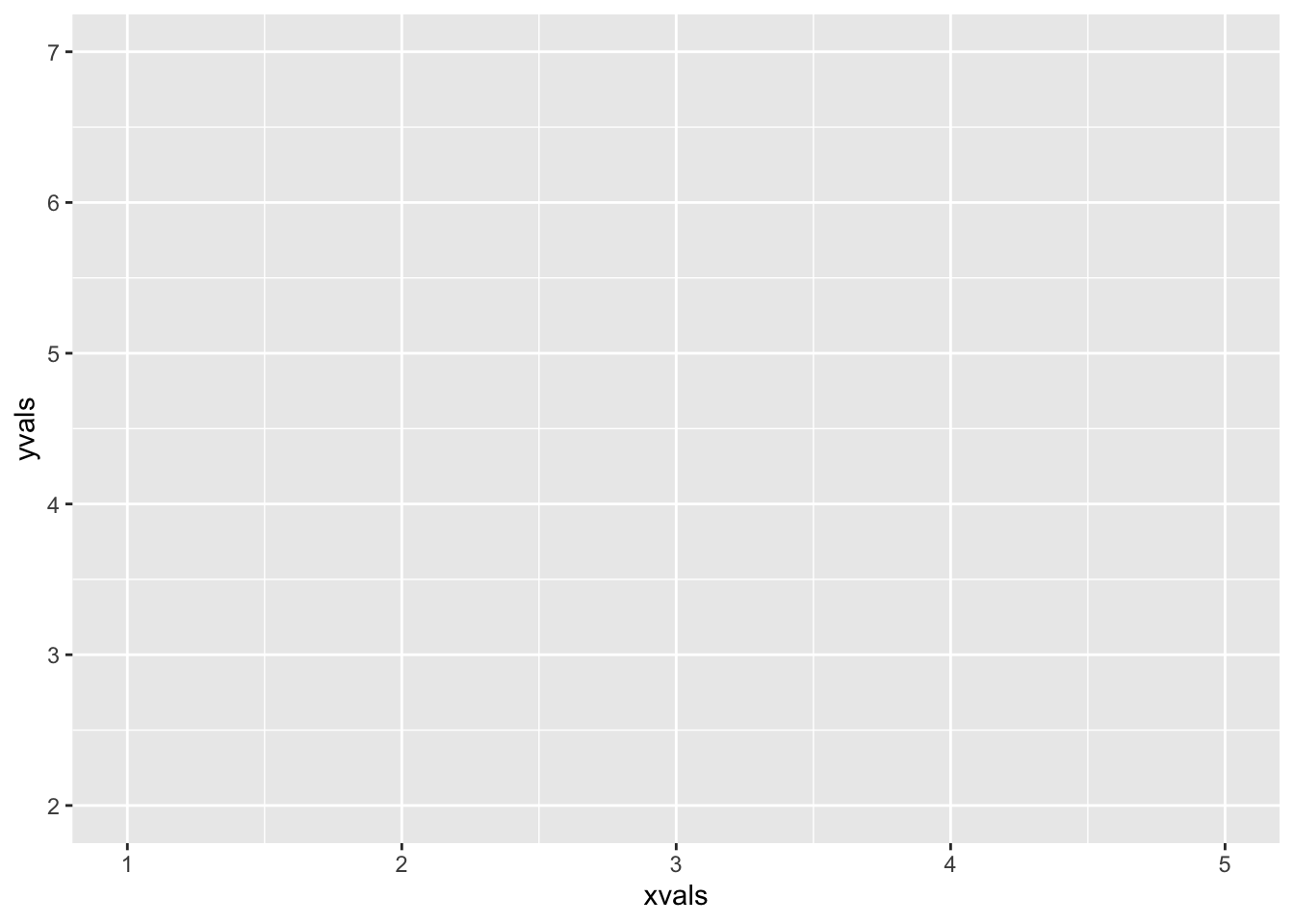
Figure 4.2: A ggplot2 plot without geoms.

The plot is blank! Why is this? Well, although ggplot() has been told what values are to be represented on the plot and where they might go, it has not yet been told how they should be shaped: it has not been told their geometry, you might say. We can add a geometry to the plot to get a picture (see Figure 4.3:

ggplot(mapping = aes(x = xvals, y = yvals)) +
  geom_point()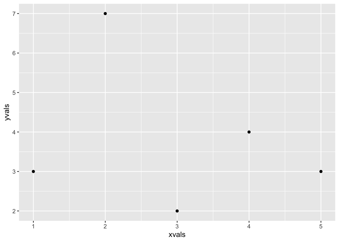

Figure 4.3: A ggplot2 plot with the point geom.

The geometry determines a lot about the look of the plot. In order to have the points connected by lines we could add geom_line() (see Figure 4.4:

ggplot(mapping = aes(x = xvals, y = yvals)) +
  geom_point() +
  geom_line()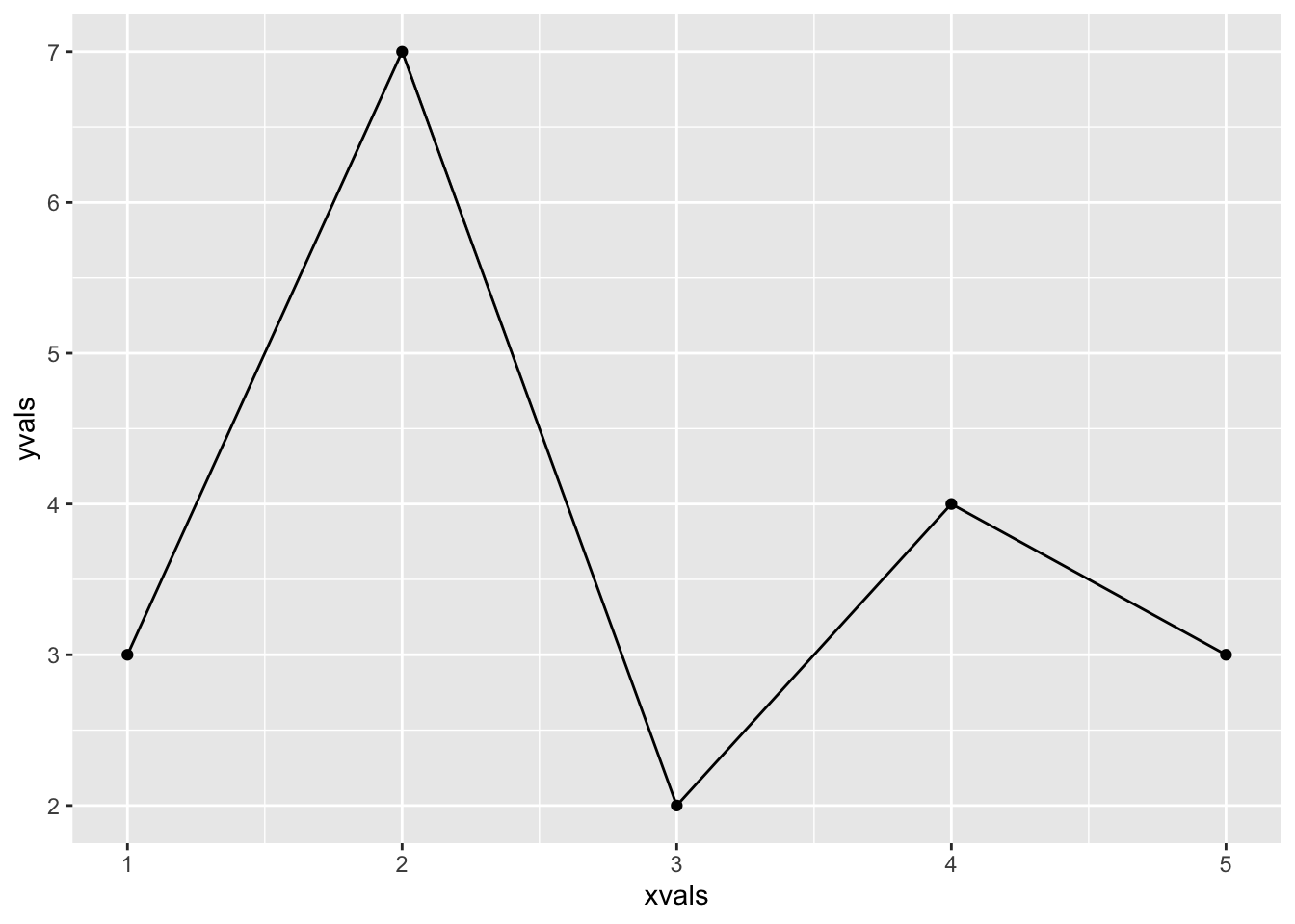

Figure 4.4: A ggplot2 plot with point and line geoms.

We’ll choose a scatter plot with connecting lines for our graph of the sequence. With a little more work we can get nice labels for the x and y-axes, and a title for the graph. Our collatz() function now looks like:

collatz <- function(n, limit = 10000) {
  # record initial number because we will change n
  initial <- n  
  numbers <- numeric(limit)
  counter <- 0
  while ( n > 1 & counter < limit) {
    counter <- counter + 1
    numbers[counter] <- n
    n <- collatzRule(n)
  }
  howMany <- min(counter, limit)
  steps <- 1:howMany
  cat("The Collatz sequence has ", howMany, " elements.\n", sep = "")
  show <- readline("Do you want to see it (y/n)?  ")
  if ( show == "y" ) {
    print(numbers[steps])
  }
  # use initial value to make plot title:
  plotTitle <- paste0("Collatz Sequence for n = ", initial)
  # make the plot
  ggplot(mapping = aes(x = steps, y = numbers[steps])) +
    geom_point() + geom_line() +
    labs( x = "Step", y = "Collatz Value at Step",
          title = plotTitle)
}

Try this version a few times, like so:

collatz(257)

It’s quite remarkable how much the sequence can rise and fall before hitting 1.

A further issue worth considering is that our collatz() function depends on the previously-defined function collatzRule(). In order for it to work correctly, R would need to be able to find the name collatzRule somewhere on the search path. If the user hasn’t already defined the collatzRule() function, then a call to `collatz() will fail.

One solution is simply to remind users of the need to define both collatzRule() and collatz() prior to running collatz(). Another solution—perhaps the kinder one—is to define the collatzRule() function in the body of collatz(). Let’s adopt this approach.

The final version of the collatz() function (with some validation thrown in for good measure) appears below.

collatz <- function(n, limit = 10000) {
  # add some validation:
  n <- suppressWarnings(as.integer(n))
  isValid <- !is.na(n) && n > 1
  if (!isValid ) {
    return(cat("Need an integer bigger than 1.  Try again."))
  }
  # define collatzRule:
  collatzRule <- function(m) {
    if ( m %% 2 == 0) {
      return(m/2)
    } else {
      return(3*m + 1)
    }
  }
  
  # On with the show!
  # Record initial number because we will change it:
  initial <- n 
  numbers <- numeric(limit)
  counter <- 0
  while ( n > 1 & counter < limit) {
    counter <- counter + 1
    numbers[counter] <- n
    n <- collatzRule(n)
  }
  howMany <- min(counter, limit)
  cat("The Collatz sequence has ", howMany, " elements.\n", sep = "")
  show <- readline("Do you want to see it (y/n)?  ")
  if ( show == "y" ) {
    print(numbers[1:howMany])
  }
  plotTitle <- paste0("Collatz Sequence for n = ", initial)
  steps <- 1:howMany
  ggplot(mapping = aes(x = steps, y = numbers[1:howMany])) +
    geom_point() + geom_line() +
    labs( x = "Step", y = "Collatz Value at Step",
          title = plotTitle)
}

4.5.9 Practice Exercises

computeSquare2 <- function(x, verbose = TRUE) {
  if ( verbose ) {
    cat("The square of ", x, " is ", x^2, ".\n", sep = "")
  }
  invisible(x^2)
}

Consider the following function:
```
computeSquare <- function(x) {
  x^2
}
```
Write a “talky” version of the above function that returns the square invisibly. It should be called computeSquare2() and should take two parameters:
- x: the number to be squared
- verbose: whether or not to cat() out a report to the Console.
Typical examples of use would be:
```
computeSquare2(4)
```
```
## The square of 4 is 16.
```
```
mySquare <- computeSquare2(6, verbose = FALSE)
mySquare
```
```
## [1] 36
```
Add some validation to the isTriangle() function so that it stops the user if one or more of the parameters x, y and z cannot be interpreted as a positive real number.
In earlier practice exercises, we made the ageReporter() function. Add some validation to it so that it rejects input unless the user provides at least one person and at least one age, with the number of people and the number of ages being equal.
Rewrite the annoying cheerleader function, using a repeat-loop instead of a while-loop.

4.5.10 Solutions to the Practice Exercises

Here’s the desired function:

computeSquare2 <- function(x, verbose = TRUE) {
  if ( verbose ) {
    cat("The square of ", x, " is ", x^2, ".\n", sep = "")
  }
  invisible(x^2)
}

Here is one approach:

isTriangle <- function(x, y, z) {
  x <- suppressWarnings(as.numeric(x))
  x <- suppressWarnings(as.numeric(x))
  x <- suppressWarnings(as.numeric(x))
  xValid <- all(!is.na(x) & x > 0)
  yValid <- all(!is.na(y) & y > 0)
  zValid <- all(!is.na(z) & z > 0)
  if (!(xValid & yValid & zValid)) {
    return(cat("Sorry, all inputs must be positive real numbers.\n"))
  }
  (x + y > z) & (x +z > y) & (y + z > x)
}

Try it out:

isTriangle(x = c(2,4,7),
           y = c(3, -4, 5),    # oops, a negative number
           z = c(6, 8, 10))

## Sorry, all inputs must be positive real numbers.

isTriangle(x = c(2,4,7),
           y = c(3, 4, 5),     # fixed it
           z = c(6, 8, 10))

## [1] FALSE FALSE  TRUE

This will do:

ageReporter <- function(people, ages) {
  ## validation:
  p <- length(people)
  a <- length(ages)
  if (p == 0) {
    return(cat("Provide at least one person!\n"))
  }
  if (a == 0) {
    return(cat("Provide at least one age!\n"))
  }
  if (!(p == a & p > 0)) {
    return(cat("Number of people must equal number of ages!\n"))
  }
  ## process:
  for (i in 1:length(people)) {
    cat(people[i], " is ", ages[i], " year(s) old.\n", sep = "")
  }
}

Try this:

cheerleader <- function(cheer) {
  for ( letter in cheer ) {
    repeat {
      call <- paste("Gimme a ", letter, "!  ", sep = "")
      response <- readline(call)
      if ( response == letter ) break
    }
  }
}

Main Ideas of This Chapter

readline() lets you interrupt the execution of commands to get input from the user at the Console.
if statements allow the code in their body to be executed provided that the governing Boolean expression evaluates to TRUE.
With if-else expressions, you run one set of expressions when the governing Boolean expression evaluates to TRUE and another set of expressions when that Boolean expression evaluates to FALSE.
You can chain if-else expressions.

The ifelse() function is not exactly flow-control, but we introduced it in this chapter because it lets you perform if-else logic on vectors of any length, like this:

height <- c(69, 67, 70, 72, 65, 63, 75, 70)
ifelse(
  height < 65,
  "short",
  "not so short"
)

## [1] "not so short" "not so short" "not so short" "not so short"
## [5] "not so short" "short"        "not so short" "not so short"

for-loops evaluate a body of expressions for each value of a given iterable.
You can use a loop to store values in a vector of results, for later use.
With a while-loop, the code in the body runs as long as the governing Boolean expression evaluates to TRUE. In order to avoid an infinite loop, you need to provide an opportunity for the governing Boolean expression to become FALSE.

Links to Class Slides

Quarto Presentations that I sometimes use in class:

Glossary

Flow Control: The collection of devices within a programming language that allow the computer to make decisions and to repeat tasks.
Condition: A Boolean expression that commences an if or while statement. If the condition evaluates to TRUE, then the code in the body of the statement will be executed. Otherwise the code will be ignored.
Index Variable: The variable in a for loop that takes on each of the values of the iterable in succession.
Iterable: The vector that provides the sequence of values for the index variable in a for loop.

Exercises

Recall that the absolute value of a number \(x\) is defined to be the number \(x\) itself if \(x \ge 0\), whereas it is the opposite of \(x\) if \(x < 0\). Thus:
- the absolute value of 3 is 3;
- the absolute value of -3 is -(-3), which is 3;
- the absolute value of -5.7 is -(-5.7), which is 5.7
- the absolute value of 0 is 0.
The absolute value is important enough that R provides the abs() function to compute it. Thus:
```
abs(-3.7)
```
```
## [1] 3.7
```
Write a function called absolute() that computes the absolute value of any given number x. Your code should make no reference to R’s abs().

Small Bonus: Write the function so that it follows the vector-in, vector-out principle, that is: when it is given a vector of numbers it returns the vector of their absolute values, like this:
```
vec <- c(-3, 5, -2.7)
absolute(vec)
```
```
## [1] 3.0 5.0 2.7
```
Write a function called pattern() that, when given any character \(x\) and any positive number \(n\), will print the following pattern to the console:
- a line with just one \(x\),
- another line with two \(x\)’s,
- another line with three \(x\)’s,
- and so on until …
- a line with \(n\) \(x\)’s, and then
- another line with \(n-1\) \(x\)’s,
- and so on until …
- a line with just one \(x\).
The function should take two arguments:
- char: the character to repeat. The default value should be "*".
- n: the number of characters in the longest, middle line. The default value should be 3.
Typical examples of use should be as follows:
```
pattern()
```
```
## *
## **
## ***
## **
## *
```
```
pattern(char = "y", n = 5)
```
```
## y
## yy
## yyy
## yyyy
## yyyyy
## yyyy
## yyy
## yy
## y
```
Hint: You already know how to cat out a line consisting of any given number of a given character:
```
char <- "*"  ## the desired character
i <- 4       ## the desired number of times
cat(rep(char, times = i), "\n", sep = "")
```
```
## ****
```
You need to make a vector that contains the desired “number of times”, for each line. Consider this method:
```
n <- 5    ## say we want 1-2-3-4-5-4-3-2-1
lineNumbers <- c(1:(n-1), n, (n-1):1)
lineNumbers
```
```
## [1] 1 2 3 4 5 4 3 2 1
```
Then you could write a for-loop that iterates over lineNumbers.
Write a function called checkerBoard() that prints outs out checkerboard patterns like this:
```
## -----------
## |*|*|*|*|*|
## -----------
## |*|*|*|*|*|
## -----------
## |*|*|*|*|*|
## -----------
## |*|*|*|*|*|
## -----------
## |*|*|*|*|*|
## -----------
```
The function should take two parameters:
- char, the character that fills the “squares” of the board. The default value should be "*".
- side, the number of rows and columns of the board. There should be no default value.
Note that the horizontal boundaries are formed by the hyphen - and the vetical boundaries are formed by the pipe character | that appears on your keyboard above the backslash \ character.

Typical examples of use should be as follows:
```
checkerBoard(char = "x", side = 3)
```
```
## -------
## |x|x|x|
## -------
## |x|x|x|
## -------
## |x|x|x|
## -------
```
Hint: Note that the number of hyphens in a boundary is always one more than twice the value of side. for example, suppose that side is 5. Then to get a row of the required hyphens, all you need is:
```
boundary <- c(rep("-", times = 2 * side + 1), "\n")
cat(boundary, sep = "")
```
```
## -----------
```
For a single row containing the character itself, you might try:
```
between <- c("|", rep(c(char, "|"), times = side), "\n")
cat(between, sep = "")
```
```
## |x|x|x|x|x|
```
In the example above, the value of char was "x".
Write a function called beerTune() that prints out the complete lyrics to the song Ninety-Nine Bottles of Beer on the Wall. You’ll recall that the song goes like this:

99 bottles of beer on the wall,

99 bottles of beer!

Take one down and pass it around:

98 bottles of beer on the wall.

98 bottles of beer on the wall,

98 bottles of beer!

Take one down and pass it around:

97 bottles of beer on the wall.

…

1 bottle of beer on the wall.

1 bottle of beer!

Take it down and pass it around:

No more bottles of beer on the wall.

Make sure to get the lyrics exactly right. For example, it’s “1 bottle”, not “1 bottles”.

Write a function called farmSong() that allows you to vary the lyrics of the song about Old McDonald’s Farm. The function should take two parameters:

animal: a character vector of names of the animals on the farm;
sound: a character vector, of the same length as the vector animal, giving the sound made by each creature in animal.

Neither parameter should have a default value.

Typical examples of use should be as follows:

farmSong(
  animal = c("cow", "hyena", "orangutan"),
  sound = c("moo", "whoop", "gorkum")
)

## Old McDonald had a farm, ee-i-ee-i-oo!
## And on this farm he had a cow, ee-iee-i-oo!
## With a moo-moo here and a moo-moo there
## Here a moo, there a moo everywhere a moo-moo,
## Old McDonald had a farm, ee-i-ee-i-oo!
## 
## Old McDonald had a farm, ee-i-ee-i-oo!
## And on this farm he had a hyena, ee-iee-i-oo!
## With a whoop-whoop here and a whoop-whoop there
## Here a whoop, there a whoop everywhere a whoop-whoop,
## Old McDonald had a farm, ee-i-ee-i-oo!
## 
## Old McDonald had a farm, ee-i-ee-i-oo!
## And on this farm he had a orangutan, ee-iee-i-oo!
## With a gorkum-gorkum here and a gorkum-gorkum there
## Here a gorkum, there a gorkum everywhere a gorkum-gorkum,
## Old McDonald had a farm, ee-i-ee-i-oo!

Note: As the above example shows, you don’t have to worry about getting “a” vs. “an” correct.

Recall the function madhavaPI() from Section 3.4. Use this function to write a function called madhavaSums() that will do the following: given a number \(n\), the function returns a vector consisting of the first \(n\) approximations to \(\pi\), using the initial terms of the Madhava series. The function should take a single argument n, whose default value is 10. It should validate the input: if the number entered is not at least 1, then the function should explain to the user that the he/she must enter a positive number, and then stop.

Here is an example of how the function should work:
```
madhavaSums(n = -3)
```
```
## You need to enter a positive integer.  Try again!
```
Here is another example:
```
madhavaSums()  # using the default value
```
```
##  [1] 4.000000 2.666667 3.466667 2.895238 3.339683 2.976046 3.283738
##  [8] 3.017072 3.252366 3.041840
```
And another:
```
madhavaSums(n = 20)
```
```
##  [1] 4.000000 2.666667 3.466667 2.895238 3.339683 2.976046 3.283738
##  [8] 3.017072 3.252366 3.041840 3.232316 3.058403 3.218403 3.070255
## [15] 3.208186 3.079153 3.200366 3.086080 3.194188 3.091624
```
R has a function called cumsum() that, when applied to any numeric vector x, will return a vector of the cumulative sums of x, meaning that for any \(i\) the \(i\)-th element of cumsum(x) is the sum of the elements of x from index 1 through index \(i\). You might have already read about cumsum() here.

Write a function called mycumsum() that does the same work on numeric vectors. It should take a single parameter named x, and it should return a vector of the cumulative sums of the elements of x. Thus, your function should do the same work ascumsum(). You may not use cumsum()` in the code for your function!

Typical examples of use should be as follows:
```
cumsum(x = c(2, 7, 5, -3, 1))
```
```
## [1]  2  9 14 11 12
```
```
cumsum(x = 4)
```
```
## [1] 4
```
```
## when numeric vector has length 0,
## return a numeric vector of length 0:
cumsum(x = numeric())
```
```
## numeric(0)
```
(*) The Subtraction Game. In this game there are two players, A and B, and a pile of \(n\) pebbles. The players take turns removing pebbles from the pile. On each turn, a player can take either one or two pebbles. The players who takes the last pebble wins the game.

It turns out that one of the players has a winning strategy. If the initial number of pebbles is a multiple of 3, then player who goes second has a winning strategy, whereas if the initial number of pebbles is not a multiple of 3 then the player who goes second has the winning strategy.

The idea for the winning strategy comes from the following observations:
- If there are 3 pebbles left and it’s the other player’s turn, then you will win. Why? Because after the other player removes pebbles there will be either 1 or 2 pebbles left. In either case you will be able to take the last pebble.
- If there are 6 pebbles left and it’s the other player’s turn, then you will win. Why? Because after the other player removes pebbles there will be either 4 or 5 pebbles left. In either case on your turn you will be able to reduce the number of pebbles to 3. The game is now in the state of the previous bullet item, where we know that you will win.
- If there are 9 pebbles left and it’s the other player’s turn, then you will win. Why? Because after the other player removes pebbles there will be either 7 or 8 pebbles left. In either case on your turn you will be able to reduce the number of pebbles to 6. The game is now in the state of the previous bullet item, where we know that you will win.
- And so on, for 12 left, 15 left, 18 left, etc.
As long as the number of pebbles left is a multiple of 3 and it’s the other player’s turn, you will win!

In this problem your task is to write a function called subtraction() that will play the Subtraction Game with a user. The function should take two parameters:
- n: the number of pebbles to begin with. The default value should be 12.
- userFirst: a logical parameter that indicates whether the user or the computer plays first. The default value should be TRUE, meaning that the user goes first.
Each time the computer plays it should announce how many pebbles it removed, and how many are left. When there are no pebbles left the computer should say who won and then quit the function.

The function should play optimally for the computer:
- if at the outset the computer has a winning strategy, then the computer should follow it and win.
- if at the outset the user has a winning strategy then the computer should watch for opportunities to win if the user departs from her winning strategy.

3 Functions

5 Turtle Graphics

4 Flow-Control

4.1 Prompting the User: readline()

4.1.1 Practice Exercises

4.1.2 Solutions to the Practice Exercises

4.2 Making Decisions: Conditionals

4.2.1 if-Statements

4.2.2 if ... else (and Absolute Value abs())

4.2.3 The ifelse() Function

4.2.4 An Application of ifelse(): Triangle Testing

4.2.5 Practice Exercises

4.2.6 Solutions to Practice Exercises

4.3 Repeating Things: Looping

4.3.1 For Loops

4.3.1.1 Iterating “By Index”

4.3.1.2 Using a Loop to Store Results

4.3.2 Breaking Out of a Loop

4.3.3 while-Loops

4.3.3.1 Application: In a Meadow, Picking Flowers

4.3.3.2 Application: A Better Guessing Game

4.3.4 Practice Exercises

4.3.5 Solutions to the Practice Exercises

4.4 Nested Loops

4.4.1 Practice Exercises

Solutions to the Practice Exercises

4.5 More in Depth

4.5.1 Validating Arguments

4.5.2 Solving the Empty-Vector Problem in for-Loops with seq_along()

4.5.3 Invisible Returns

4.5.4 Switch

4.5.5 For-Loop Caution

4.5.6 Skipping Ahead in a Loop

4.5.7 Repeat

4.5.8 Extended Example: The Collatz Conjecture

4.5.9 Practice Exercises

4.5.10 Solutions to the Practice Exercises

Main Ideas of This Chapter

Links to Class Slides

Glossary

Exercises

4.1 Prompting the User: `readline()`

4.2.1 `if`-Statements

4.2.2 `if ... else` (and Absolute Value `abs()`)

4.2.3 The `ifelse()` Function

4.2.4 An Application of `ifelse()`: Triangle Testing

4.3.3 `while`-Loops

4.5.2 Solving the Empty-Vector Problem in `for`-Loops with `seq_along()`