15.7 Generic-Function OO
We now turn to the second major type of object-oriented programming that is supported by R, namely: generic-function OO.
15.7.1 Motivating Examples
We begin by revisiting the task of printing to the console.
Recall that whenever we type the name of an object into the console and press Enter, R interprets the input as a call to the print() function. Consider, for example, printing some portion of m111survey from the bcscr package:
df <- bcscr::m111survey[1:5, c("height", "weight_feel")]If we want to print df, then either of the following two statements accomplish the same thing:
print(df) ## explicit directive to print results to Console## height weight_feel
## 1 76 1_underweight
## 2 74 2_about_right
## 3 64 2_about_right
## 4 62 1_underweight
## 5 72 1_underweightdf ## R implicity calls print() at top-level## height weight_feel
## 1 76 1_underweight
## 2 74 2_about_right
## 3 64 2_about_right
## 4 62 1_underweight
## 5 72 1_underweightBoth expressions, as we learned long ago, involve a call to the print() function.
But let’s think a bit more deeply about what we see in the Console.
It is tempting to think of the above printouts as simply what the object df is. But that’s not quite right. In truth, it merely reflects how R represents df to us in the console. R was programmed to represent df in spreadsheet-format—with variables along columns, individuals along rows, and with handy row-numbers supplied—because human users are accustomed to viewing data tables in that way.
But now let us turn df into a list:
lst <- as.list(df)
str(lst)
## List of 2
## $ height : num [1:5] 76 74 64 62 72
## $ weight_feel: Factor w/ 3 levels "1_underweight",..: 1 2 2 1 1And let’s print lst:
lst # same as print(lst)## $height
## [1] 76 74 64 62 72
##
## $weight_feel
## [1] 1_underweight 2_about_right 2_about_right 1_underweight 1_underweight
## Levels: 1_underweight 2_about_right 3_overweightWe get the familiar output for a list whose elements are named. Users don’t expect lists to be represented in the console in spreadsheet-style format, even if the elements of the list happen to be vectors that are all of the same length. They expect a more “neutral” representation, and R delivers one.
Printing to the console is a common task. It appears, however, that the method by which that task is performed depends on the type of object that is input to the print() function:
- If your object is a data frame,
print()behaves one way. - If your object is a list, print does something else.
Since the behavior of print() depends on the type of object involved in the operation of printing, you could say that it exhibits polymorphism. .
In fact it is the class of the object given to print() that determines the method that prints() employs. The class of an R-object can be accessed with the class() function :
class(df)## [1] "data.frame"class(lst)## [1] "list"How does the class of df determine the method used for printing? To see how this is done, look at the code for the print() function:
print## function (x, ...)
## UseMethod("print")
## <bytecode: 0x108da3d40>
## <environment: namespace:base>The body of the print() consists of just one expression: UseMethod("print"). On the fact of it, this doesn’t seem to accomplish anything! In reality, though, a lot is taking place under the hood. Let’s examine what happens, step-by-step, when we call print(df).
The data frame
dfis assigned to the parameterxin theprint()function.We call
UseMethod("print").From
help(UseMethod)we learn thatUseMethod()takes two parameters:generic: a character string that names the task we want to perform. In this casegenerichas been set to “print.”object: this is an object whose class will determine the method that will be “dispatched,” i.e., the method that will be used to print the object to the console. By default this is the first argument in the enclosing functionprint(), soobjectgets set to the data framedf.
Control has now passed to the
UseMethod()function, which searches for a suitable method for printing an object of classdata.frame. It does this by pasting together “print” (the argument togeneric) anddata.frame(the class of the objectdfit was given) with a period in between, getting the string “print.data.frame.” A search is now conducted for a function having that name.The function
print.data.frame()will be found. We can tell because it appears on the list of available “methods” forprint(). Themethods()function will give us the complete list of available methods, if we likemethods("print")## [1] print,ANY-method ## [2] print,diagonalMatrix-method ## [3] print,sparseMatrix-method ## [4] print.abbrev* ## [5] print.acf* ## ... ## [87] print.data.frame <== Here it is! ## [88] print.data.table ## ...R now calls the
print.data.frame(), passing indf. The data frame is printed to the console.When
UseMethod()completes execution, it does not return control to the enclosing functionprint()from which it was called. The work of printing is done, so R arranges for control to be passed back to whomever calledprint()in the first place.
It is interesting to note that the very act of “printing out” the print function, which we did earlier in order to see the code for the function, involved a search for a printing method:
print # this is equivalent to print(print)## function (x, ...)
## UseMethod("print")
## <bytecode: 0x108da3d40>
## <environment: namespace:base>In the call print(print), R looked at the class of print(), and found that it was of class function:
class(print)## [1] "standardGeneric"
## attr(,"package")
## [1] "methods"R then searched for a method called print.function and found one. Note that this method gives the sort of output to the console that would be helpful to a user:
- the code for the function;
- the location of the function in memory:
0x108da3d40; - the environment in which the function was defined (the package base).
Things go a little bit differently in the call to print(lst). The class of lst is list, but when you search the results of methods(print) you won’t find a print.list() method; accordingly R uses a fall-back method called print.default(). This is why the console-output for lists looks so “neutral.”
15.7.2 Terminology
The print() function is an example of a generic function. A generic function is simply a function that performs a common task by dispatching its input to a particular method-function that is selected on the basis of the class of the input to the generic function. Languages that use generic functions are said to support generic-function OO.
In message-oriented OO, objects own their own methods, and the way a task is performed depends on the class of the object that is invoked to perform the task. Generic-function OO, which is most commonly found in languages that support functional programming, puts more stress on functions: the generic function “owns” the methods in the sense that it acts as the central dispatcher, assigning a method function to perform a given task. In a bit of a reversal to message-passing OO, the method selected in generic-function OO depends on the class of the input-object to the generic, not on the class of the generic that was called to perform the task.
We should also mention that R actually has two ways to implement generic-function OO:
- S3 classes;
- S4 classes.
S3 classes were the first to be implemented, and to this day they are more commonly-used than S4 classes are. Therefore they are the implementation we will study. (S4 classes tend to be used by programmers in applications where there significant concern that the rules for formation of S3 classes aren’t strict enough.)
15.7.3 Common Generic Functions
There are three very commonly-used generic functions in R:
print(), which we have examined already;summary();plot().
Each of these generics is associated with a large number of method-functions. This is a great advantage to the casual user of R: one has to know only a few R-commands in order to acquire useful information about a wide variety of R-objects.
It is always a good idea to “try out” generic functions on objects you are using. You never know if the authors of R, or of a contributed package you have attached, may have written methods that are precisely tailored to that object.
Here are some example of the versatile, polymorphic behavior of the generic function summary():
heights <- df$height # vector of class "numeric"
summary(heights)
## Min. 1st Qu. Median Mean 3rd Qu. Max.
## 62.0 64.0 72.0 69.6 74.0 76.0feelings <- df$weight_feel # has class "factor"
summary(feelings)## 1_underweight 2_about_right 3_overweight
## 3 2 0summary(df) # summarizing object of class "data.frame"## height weight_feel
## Min. :62.0 1_underweight:3
## 1st Qu.:64.0 2_about_right:2
## Median :72.0 3_overweight :0
## Mean :69.6
## 3rd Qu.:74.0
## Max. :76.0summary(lst)## Length Class Mode
## height 5 -none- numeric
## weight_feel 5 factor numericIt is interesting also to see how R’s plot() (from package base) reacts to various types of input. See the Figure 15.2
x <- seq(-3, 3, by = 0.01)
plot(x^2)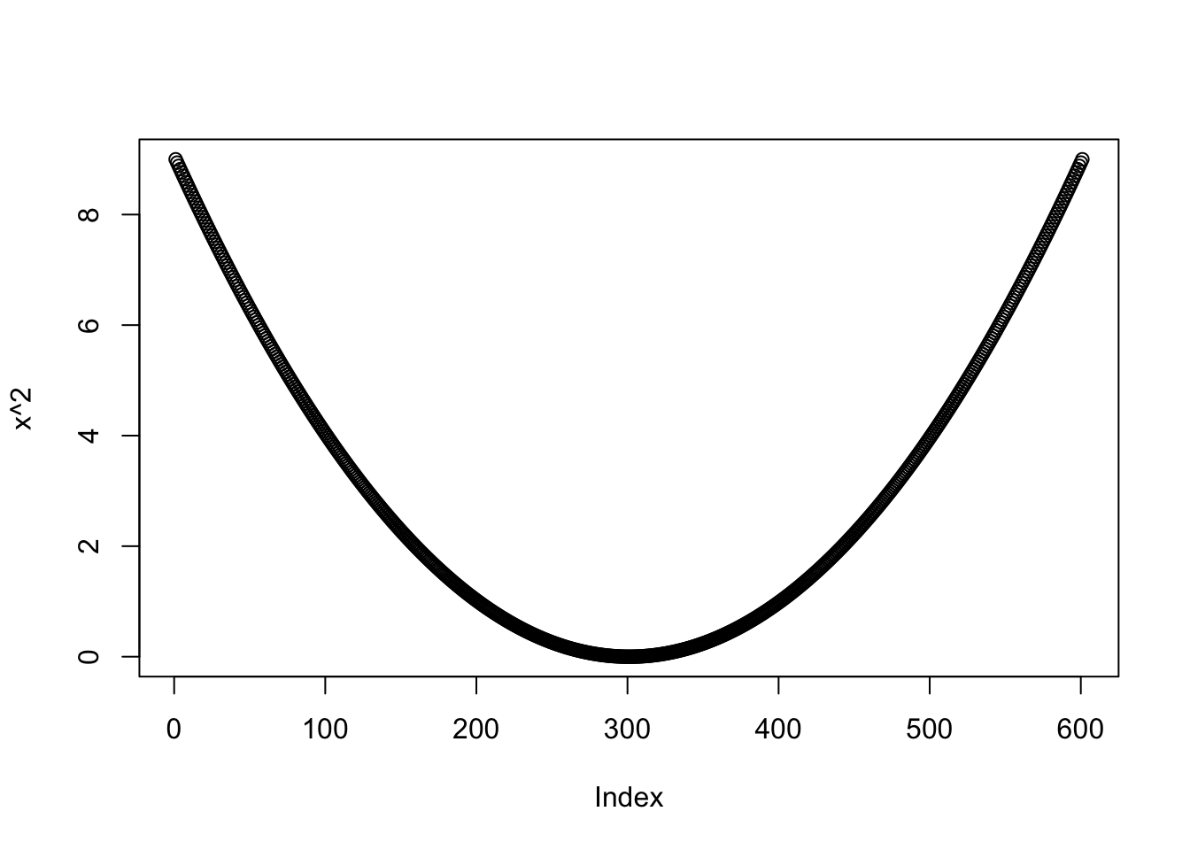
Figure 15.2: Our vector graphed as a parabola!
15.7.4 Writing Your Own Methods
As you advance in your programming skills, you will transition from writing programs to help you accomplish your own tasks to writing programs that help others—who are not as proficient in programming as you are—get some of their work done. Since casual users of R often become accustomed to generic functions as providers of useful information about many types of R-objects, you might find yourself writing methods for one or more of the common generic functions. In this Section will we will practice the art of method-writing: we will write some method-functions to report on the results of a simulation.
Recall the problem from Section 6.6 about estimating the expected number of uniform random numbers one must create until their sum exceeds a specified target-number. Let’s rewrite the simulation function so that it returns an object of a special class. We will then write print and plot methods that permit a user to obtain information about the results of any simulation that was performed.
First of all, let’s rewrite numberNeededSim():
numberNeededSim <- function(target = 1, reps = 1000,
                            seed = NULL) {

  # set the seed if none is provided
  if (!is.null(seed)) {
    set.seed(seed)
  }

  numberNeeded <- function(target) {
    mySum <- 0
    count <- 0
    while (mySum < target) {
      number <- runif(1)
      mySum <- mySum + number
      count <- count + 1
    }
    count
  }

  needed <- numeric(reps)
  for (i in 1:reps) {
    needed[i] <- numberNeeded(target)
  }
  results <- list(target = target, sims = needed)
  class(results) <- "numNeededSims"
  results
}
In the above code you will note that there is no longer a parameter table to permit printing of a table to the console. Also, nothing at all is cat-ed to the console. Instead we return only a list with two named elements:
target: the target you want your randomly-generated numbers to sum up to;sims: the number of numbers required to sum to the target, in each repetition of the simulation.
The class of the returned list is set as “numNeededSims.”
Next, we write a print-method function. Its name must be print.numNeededSims. All of the table output and cat-ing to the console goes here:
print.numNeededSims <- function(x) {
  cat("The target was ", x$target, ".\n", sep = "")
  sims <- x$sims
  reps <- length(sims)
  cat("Here is a table of the results, based on ", reps,
    " simulations.\n\n",
    sep = ""
  )
  tab <- prop.table(table(sims))

  # for sake of pretty output,
  # remove "sims" variable name from top of table printout
  colNames <- dimnames(tab)
  names(colNames) <- NULL
  dimnames(tab) <- colNames

  print(tab)
  cat("\n")
  cat("The expected number needed is about ",
    mean(sims), ".\n",
    sep = ""
  )
}
Finally, let’s write a plot method. Its name must be plot.numNeededSims. This method will produce a bar graph of the results of the simulations. We’ll use the ggplot2 plotting package, so we should stop if the user hasn’t installed and attached ggplot2.
plot.numNeededSims <- function(x) {
  if (!"package:ggplot2" %in% search()) {
    return(cat("Need to load package ggplot2 in order to plot."))
  }

  sims <- x$sims
  # for a good bar-plot, convert numerical vector sims
  # to a factor with appropriate levels
  levels <- min(sims):max(sims)
  sims <- factor(sims, levels = levels)

  df <- data.frame(sims)
  plotTitle <- paste0("Results of ", length(sims), " Simulations")
  # in the code below, scale_x_discrete(drop = f) ensures that
  # even if there are no values in sims for a particular level it
  # will still appear in the plot as a zero-height bar
  ggplot(df, aes(x = sims)) + geom_bar() + scale_x_discrete(drop = FALSE) +
    labs(x = "Number Needed", title = plotTitle)
}
Let’s give it a try:
numberNeededSim(reps = 10000, seed = 4040)## The target was 1.
## Here is a table of the results, based on 10000 simulations.
##
## 2 3 4 5 6 7
## 0.4974 0.3354 0.1253 0.0339 0.0068 0.0012
##
## The expected number needed is about 2.7209.The print function was called implicitly, so we got useful output to the console.
It’s also possible to save the results somewhere, for example:
results <- numberNeededSim(reps = 10000, seed = 4040)
str(results)
## List of 2
## $ target: num 1
## $ sims : num [1:10000] 3 2 2 2 3 3 4 2 2 5 ...
## - attr(*, "class")= chr "numNeededSims"Then it’s possible for the user to recall specific features of the results, for example:
results$target # get just the target number## [1] 1If we wanted the printout we could just say:
results## The target was 1.
## Here is a table of the results, based on 10000 simulations.
##
## 2 3 4 5 6 7
## 0.4974 0.3354 0.1253 0.0339 0.0068 0.0012
##
## The expected number needed is about 2.7209.For a plot we can use the plot() generic. The resulting graph appears as Figure 15.3.
plot(results)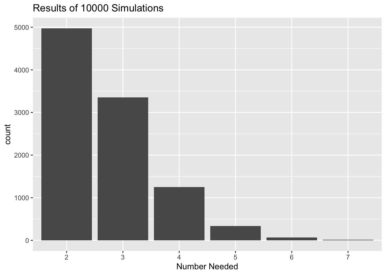
Figure 15.3: Results of the Number-Needed simulation.
15.7.5 Writing a Generic Function
Generic functions are most useful when they correspond to tasks that are so commonly performed that many methods are written for them, so that users get in the habit of “trying out” the generic on their object. As a consequence, the vast majority of method-functions are written for currently-existing, very well-known generics like print(), summary() and plot(). It doesn’t make a lot of sense to write generics that will have only a few methods attached to them. Nevertheless, it’s highly instructive to see how generics do their work, so as an example we’ll write a new generic, along with a couple of method functions.38
First let’s create some objects with special classes. Here are two objects of class “cartesianPoint.” Our intention is that they correspond to points on the plane, represented with the standard \(x\) and \(y\) Cartesian coordinates.
point1 <- list(x = 3, y = 4)
class(point1) <- "cartesianPoint"
point2 <- list(x = 2, y = 5)
class(point2) <- "cartesianPoint"
It is also possible to represent a point on the plan with polar coordinates. The elements of a polar coordinates representation are:
- \(r\): a non-negative real number that gives the distance from the origin to the point;
- \(\theta\): the angle measure (in radians) between the positive \(x\)-axis and ray from the origin to the point.
point3 <- list(r = 2, theta = pi / 2)
point4 <- list(r = 1, theta = pi)
class(point3) <- "polarPoint"
class(point4) <- "polarPoint"
In the definition above, point3 is the point that lies at \(\pi/2\) radians (90 degrees) counter-clockwise from the positive \(x\)-axis. That means that it lies along the positive \(y\)-axis. It is 2 units from the origin, so in Cartesian coordinates it would be written as \((0,2)\). Similarly, point4 would be written in Cartesian coordinates as \((-1,0)\), since it lies one unit from the origin along the negative \(x\)-axis.
Now let us suppose that we would like to find the \(x\)-coordinate of a point. For points of class cartesianPoint this is pretty simple:
point1$x # gives x-coordinate## [1] 3If the point is given in polar coordinates, we must convert it to Cartesian coordinates. You may recall the conversion formulas from a previous trigonometry class. To get \(x\), use:
\[x = r\cos \theta.\]
To get \(y\), use:
\[y = r\sin \theta.\]
Thus, to find the \(x\)-coordinate for point3, work as follows:
point3$r * cos(point3$theta)## [1] 1.224647e-16The result is 0 (to a tiny bit of round-off error).
We now write a generic function xpos() for the \(x\)-coordinate:
xpos <- function(x) {
  UseMethod("xpos")
}
We need to write our method functions, one for each point class:
xpos.cartesianPoint <- function(point) {
  point$x
}

xpos.polarPoint <- function(point) {
  point$r * cos(point$theta)
}
Now we can feed points of either class into the generic xpos() function:
xpos(point2)## [1] 2xpos(point4)## [1] -1The generic we write is drawn from an example provided in the official R Languge Definition (R Core Team (2017)), written by the developers of R.↩︎