15 Object-Oriented Programming in R

repeat {
  coffeeMug$drinkFrom()
  workTask$execute()
  if (coffeeMug$empty()) {
    if (coffeePot$empty()) {
      coffeePot$make()
    }
    coffeeMug$fill()
  }
  if (workTask$done()) {
    break
  }
}

Our journey with R began in the Procedural Programming paradigm. In the last Chapter we learned about R’s extensive support for the more modern paradigm known as Functional Programming. In the present Chapter we will explore the ways in which R supports a third modern programming paradigm: Object-Oriented Programming.

15.1 The Object-Oriented Programming Paradigm

We started out with Procedural Programming, which draws a distinction between data and procedures. Data provides our information, and procedures solve problems by manipulating data into new forms.

Functional Programming puts functions at the center of attention. As much as possible, procedures are wrapped up in function calls, and by their status as first-class citizens (data) functions become king. Everything that happens is a result of function calls on data–where the data can include other functions.

You could say that Object-Oriented Programming reverses the point of view, attempting to put objects–conceived as complex forms of data–at the center of attention.

There are two major types of Object-Oriented (OO) Programming:

Message-Passing OO
Generic-Function OO

Message-Passing OO is the type of OO Programming that programmers usually associate with the term “object-oriented”, and since it is the type that you will meet most frequently in other languages that support OO-programming we will discuss it first. Generic-Function OO is actually the older type of OO Programming. Although it is very important for understanding some aspects of how R works, it is met with less frequently in other major programming languages, so we will defer discussion of it until Section 15.7. Accordingly, the following introductory remarks pertain only to message-passing OO.

Objects in the world about us are indeed complex entities: they have particular features. Some of these features they have in virtue of the kind of object that they are, and others are features–attributes–that they have on their own, as individuals. And they can do various things. Again, some of the things they do are things that they do simply because of the kind of thing they are, and others things they do might be unique to them.

Consider a typical object: my dog, for example. He has various attributes: his name is Beau, he has four legs, he weighs about 50 pounds, his hair is black. And he does various things—he has various methods, let’s say, for making his way through life. For example, when we are out of the house he lies in the sofa, when we are home he lies on the floor. He barks. He eats. He annoys cats.

Some of his attributes and methods Beau has simply in virtue of being the kind of thing that he is. He is, after all, a dog—a member of the class Dog, let’s say—and so like all other dogs he will have four legs and he will be able to bark and to annoy cats. Of course all dogs are animals—members of the more general class Animal, let’s say—and all animals eat, so as an animal Beau inherits the method known as eating. Of course all animals are material beings—members of the even-more general class Being, let’s say—and all beings have a weight, and thus Beau has a weight, but the particular value of that weight—50 pounds—is determined by the way he has lived his life thus far. Other dogs, animals and material beings have a weight, but they won’t necessarily have the same weight as Beau.

What emerges from this discussion is an (admittedly oversimplified) view of the world as a collection of complex objects. These objects are related to one another in systematic ways–related closely when they are, for instance, both Dogs, and more distantly, as when one is a Dog and another is a Cat. And these objects can act on themselves and on each other in various ways, through their methods.

The idea of Object-Oriented Programming is that since we are so used to viewing the world as a collection of objects that are constituted of various attributes and methods and that are related to one another through membership in classes of varying levels of generality, then it might help us to be able to view a computer program similarly—as a collection of objects thus constituted and thus related to one another.

Like many other modern programming languages, R provides considerable support for the Object-Oriented paradigm. In fact it provides that support in two different formats:

Reference Classes
R6 Classes

Reference Classes are a relatively recent introduction to R. R6 Classes are a simple and lightweight version of Reference Classes. They are not a part of the core of R—they are enabled by a contributed R-package—but they are quite useful as an introduction to object-oriented programming. Accordingly, we will work with them in this Chapter.

15.2 Reference Classes with Package R6

The package R6 (Chang 2021) provides access to R6 classes. You will need to attach it:

library(R6)

We’ll get started by creating a miniature computerized world of objects that is based on characters from the Wizard of Oz.

15.2.1 Defining a Class

Construction of the object-world begins with the definition of classes. A class is simply a general prototype on the basis of which actual objects may be created.

Let’s define the class Person. This is accomplished with the R6Class() function:

Person <- R6Class(
  classname = "Person",
  public = list(
    name = NULL,
    age = NULL,
    desire = NULL,
    initialize = function(name = NA, age = NA, desire = NA) {
      self$name <- name
      self$age <- age
      self$desire <- desire
      self$greet()
    },
    set_age = function(val) {
      self$age <- val
      cat("Age of ", self$name, " is:  ", val, ".\n", sep = "")
    },
    set_desire = function(val) {
      self$desire <- val
      cat("Desire of ", self$name, " is:  ", val, ".\n", sep = "")
    },
    greet = function() {
      cat(paste0("Hello, my name is ", self$name, ".\n"))
    }
  )
)

Let’s analyze the above code. The function R6Class() has a quite a few parameters, but the two with which we will concern ourselves the most are:

classname: the name we propose to give to the class;
public: a list of members of the class that are “public” in the sense that they can be accessed and used outside of the class.³⁵ Members are of two types:
- attributes: the objects name, age and desire. Currently these have value NULL, but they can be given other values later on. What makes then attributes, though, is that they will not be given a function as a value.
- methods: these are members of the class that are functions. You can think of a “method” as a particular way of performing a common task that could be performed in many different ways. The four methods you see in Person are:
  - initialize: This is a function that will be run whenever a new object of class Person is created. As we can see from its arguments, it will be possible to give values to the attributes name. age and desire when this function is called.
  - set_age and set_desire are functions that allow a user to set or to change the value of age and desire for an object of class Person.
  - greet: a function that will permit an object of class Person to issue a greeting.

Note the use of the term self in the code for the methods of the class. When a method is called on an object, the term self will refer to the object on which the method is being called. Hence, for example, in the code for greet the term self$name will evaluate to the name of the person who issues the greeting.

15.2.2 Instantiation: Initializing Objects

On its own there is not much that a class can do. For anything to happen we need to create a particular individual: an object of class Person. Creation of an object having a particular class is called instantiation.

Every class comes with a method—not mentioned in the definition of the class—called new(). This method, when called on the Class, instantiates an object of the class by running the initialize() function. Let’s create a person named Dorothy and store this new object in the variable dorothy:

dorothy <- Person$new(
  name = "Dorothy", age = 12,
  desire = "Kansas"
)

## Hello, my name is Dorothy.

Note how the dollar-sign is used to indicate the calling of the new() method on the class Person. Note also that the arguments of new() are the arguments of initialize(): that’s because the new() method actually runs initialize() as part of its object-creation process.

We can get a look at dorothy by printing her to the console:

dorothy

## <Person>
##   Public:
##     age: 12
##     clone: function (deep = FALSE) 
##     desire: Kansas
##     greet: function () 
##     initialize: function (name = NA, age = NA, desire = NA) 
##     name: Dorothy
##     set_age: function (val) 
##     set_desire: function (val)

We get the basic information on Dorothy, including also an indication that she can be cloned (copied). We’ll discuss cloning later.

We can instantiate as many people as we like. The code below for example, establishes scarecrow as a new instance of Person:

scarecrow <- Person$new(
  name = "Scarecrow", age = 0.038,
  desire = "Brains"
)

## Hello, my name is Scarecrow.

In The Wizard of Oz, Scarecrow is only two weeks old when Dorothy meets him, so his age is set at $2/52 \approx 0.038$ years.

15.2.3 Getting and Setting Attributes

If we would like to change Dorothy’s age, we can do so by calling the set_age() method on her:

dorothy$set_age(13)

## Age of Dorothy is:  13.

dorothy$age

## [1] 13

We can also set Dorothy’s age directly, by regular assignment:

dorothy$age <- 14

dorothy$age

## [1] 14

The effect is the same as when we use set_age() except that we don’t get a report to the console.

15.2.4 Calling Methods

We have seen that in order to call a method on an object, you follow the format:

object$method()

Thus, we can ask dorothy to issue a greeting:

dorothy$greet()

## Hello, my name is Dorothy.

In the syntax for calling methods, we see one aspect of “message-passing”: dorothy$greet() essentially passes a message to dorothy: “Please call your greet() method!”

15.2.5 Holding a Reference, not a Value

R6 objects operate by what are known in computer programming as reference semantics. This means that when the assignment operator is used to assign an R6 object to a variable, the new variable holds a reference to that object, not a copy of the new object.

This is in contrast value semantics, which is the way assignment usually works in R. In value semantics, R a distinct copy of the value of the assigned object is created, and the new variable refers to that copy. Below is an example of the familiar value semantics in action:

a <- 10
b <- a
b <- 20
a

## [1] 10

b has been changed to 20, but that change did not affect a, which keeps its initial value of 10.

We can use the function address() from the package pryr (Wickham 2023) to track what is happening behind the scenes. address() will tell us the current location in memory of the value corresponding to a name. Let’s repeat the above process, but use address() to see where the values are stored:

a <- 10
pryr::address(a)

## [1] "0x7fd57297a9c0"

The value 10 is stored in the memory address given above. Next, let’s create b by assignment from a:

b <- a
pryr::address(b)

## [1] "0x7fd57297a9c0"

For the moment b points to the same place in memory as a does, so it will yield 10:

## [1] 10

We can use b for other operations; for example, we can add 30 to it:

b + 30

## [1] 40

But for now b still points to the same place in memory that a does:

pryr::address(b)

## [1] "0x7fd57297a9c0"

But now let’s assign a new value to b:

b <- 20
pryr::address(b)

## [1] "0x7fd5696e2398"

Aha! b now points to a new location in the computer’s memory! That’s because R saw that the assignment operator was going to change the value of b. Since b has value semantics, R knows to set aside a new spot in memory to contain the value 20, and to associate the name b with that spot. That way, the new b won’t interfere with a, which points to the same old spot in memory and thus remains 10:

pryr::address(a)

## [1] "0x7fd57297a9c0"

## [1] 10

On the other hand, R6 objects have reference semantics. We can see this in action with the following example. First, let’s check on dorothy’s age:

dorothy$age

## [1] 14

Let’s now create dorothy2 by assignment from dorothy:

dorothy2 <- dorothy

Let’s check the memory locations:

c(pryr::address(dorothy), pryr::address(dorothy2))

## [1] "0x7fd570112770" "0x7fd570112770"

As with a and b, the two names initially point to the same place in memory.

Now let’s change the age of dorothy2 to 30:

dorothy2$age <- 30

Let’s check the age of dorothy:

dorothy$age

## [1] 30

Whoa! Changing the age of dorothy2 changed the age of dorothy! That’s because of the reference semantics: dorothy2 continues to be associated with the same spot in memory as dorothy, even after we begin to make changes to it:

c(pryr::address(dorothy), pryr::address(dorothy2))

## [1] "0x7fd570112770" "0x7fd570112770"

15.2.6 Cloning an Object

For the sorts of complex objects created by R6 classes, reference semantics can be a useful feature. But what if we want a new and truly distinct copy of an R6 object? For this we need the clone() method that was alluded to earlier:

dorothy2 <- dorothy$clone()
dorothy2

## <Person>
##   Public:
##     age: 30
##     clone: function (deep = FALSE) 
##     desire: Kansas
##     greet: function () 
##     initialize: function (name = NA, age = NA, desire = NA) 
##     name: Dorothy
##     set_age: function (val) 
##     set_desire: function (val)

dorothy2 looks just like dorothy. However, the name dorothy2 does not point to the same place in memory:

c(pryr::address(dorothy), pryr::address(dorothy2))

## [1] "0x7fd570112770" "0x7fd55bfc2d20"

Accordingly, changes to dorothy2 will no longer result in changes to dorothy:

dorothy2$age <- 100
dorothy$age

## [1] 30

You should know that if one or more of the members of an object is itself an object with reference semantics (such as an instance of an R6 class), then a copy produced by clone() will hold a reference to that same member-object, not a separate copy of the member-object. In such a case if you still want a totally separate copy, you will have to consult the R6 manual on the topic of “deep cloning.”

15.3 Inheritance

Earlier we mentioned that in the real world an object may possess a property in virtue of being the particular kind of thing that it is, or it may possess that property in virtue of being a member of some more general class of things. Thus a dog can eat, not because it is a dog per se, but because it is an animal. You could say that dogs “inherit” the capacity to eat from the class Animal.

Most object-oriented frameworks allow for some type of inheritance between classes, and R6 is no exception. In the Wizard of Oz lions appear to be a special type of person: after all, they can speak, and they have desires. Accordingly, we should create a new class Lion that inherits from the class Person:

Lion <- R6Class("Lion",
  inherit = Person,
  public = list(
    weight = NULL,
    set_weight = function(val) {
      self$weight <- val
      cat(self$name, " has weight:  ", val, ".\n", sep = "")
    },
    greet = function() {
      cat("Grr!  My name is ", self$name, "!", sep = "")
    }
  )
)

The key to inheritance is the new argument in the code above:

inherit = Person

The impact of this additional argument is that any instance of the class Lion will possess by default all of the attributes and methods of class Person, in addition to the new attributes and methods (weight, set_weight, and greet) specified explicitly in the definition of class Lion. Of these three explicitly-defined members:

weight and set_weightwere not already in Person, so they are simply added on as members of Lion;³⁶
greet was already a member of Person, but the new specification of greet in the definition of Lion overrides the old one. Any instance of class Lion will greet us according to the code for greet() given in the definition of Lion. (Objects that are instances of the class Person, however, will go on greeting us just as they always have done.)

Let’s verify all of this by making an instance of class Lion:

cowardlyLion <- Lion$new(
  name = "Cowardly Lion",
  age = 18, desire = "courage"
)

## Grr!  My name is Cowardly Lion!

Since the definition of class Lion did not specify a new method of initialization—we could have asked for this, but chose not to—the instantiation of a lion won’t set its weight. We will have to do that separately:

cowardlyLion$set_weight(350)

## Cowardly Lion has weight:  350.

Inheritance is an very effective way to re-use code and to keep code for a particular function in one place. Once we have written methods for some class X, those methods will be available to any objects that are instances of classes that inherit from class X. Hence there is no need to repeat the code in the definition of the inheriting classes. Later on if we need to modify one of of the class X methods, we need only make the change in class X: we don’t have to worry about changing it in all of the classes that inherit from X.

Let’s ask cowardlyLion to greet us:

cowardlyLion$greet()

## Grr!  My name is Cowardly Lion!

As expected, the greeting includes a growl, since the greet() method for class Lion overrides the growl-less greet() method that it would have otherwise inherited from class Person. We also see a fundamental aspect of message-passing OO at work:

The method used for determining how a particular task is performed is determined by the class of the object that is asked to perform the task.

Here we have the task of greeting, which is common to objects of class Person and to objects of class Lion. That task may be performed with or without a growl. Precisely how it is performed—the method that is selected for carrying out the task—depends upon the class of the object that performs the greeting: an object of class Person will greet you without a growl, whereas an object of class Lion will greet you with a growl.

The common task of greeting may be performed in different ways, depending upon the class of the object involved in the task. This is an example of what programmers call polymorphism. The term “polymorphism” comes from a Greek word that means “many forms”, and it refers to a task being performed differently depending on the class of the object involved. Polymorphism makes programming a bit easier: you only have to remember the name of the one common task. Invoke it on an object and you can rest assured that the task will be performed in the way that is right and proper to that object.

15.4 Adding Members to a Class

Sometimes we need to add or to modify a member of a class, after we have defined that class. Every class comes with a set() method that allows us to do this. For example, suppose that we would like our people to have a favorite color:

Person$set("public", "color", NA, overwrite = TRUE)

We now see that color is now one of the public members of class Person:

Person

## <Person> object generator
##   Public:
##     name: NULL
##     age: NULL
##     desire: NULL
##     color: NA
##     initialize: function (name = NA, age = NA, desire = NA) 
##     set_age: function (val) 
##     set_desire: function (val) 
##     greet: function () 
##     clone: function (deep = FALSE) 
##   Parent env: <environment: R_GlobalEnv>
##   Locked objects: TRUE
##   Locked class: FALSE
##   Portable: TRUE

In the above call to set, the argument overwrite = TRUE was not strictly necessary, since color did not previously exist as a member of Person. If you are developing a program, though, and you find yourself repeatedly running a piece of code that sets a new member for a class, it’s useful to have overwriting turned on.

While we are at it. let’s write a special set_color() method:

Person$set("public", "set_color", function(val) {
  self$color <- val
  cat(self$name, " has favorite color: ", val, ".\n", sep = "")
}, overwrite = TRUE)

You might think that we can now set a favorite color for dorothy:

dorothy$set_color("blue")

Error: attempt to apply non-function

Why did this not work? It turns out that when you add a new member to a class it is only available to instances of the class that are created after the new member is added to that class. If we create a new instance of Person, the Good Witch Glinda, let’s say, then we should be able to give her a favorite color:

glinda <- Person$new("Glinda", "500", "the good of all")

## Hello, my name is Glinda.

glinda$set_color("blue")

## Glinda has favorite color: blue.

15.5 Method Chaining

In this Section we will explore a concise and convenient device for calling multiple methods on an object. The device is known as method chaining.

In order to illustrate method chaining, we’ll extend the class Lion a bit, with some new attributes and new methods. First of all, we’d like to add a data frame consisting of possible animals on which a lion might prey. The data frame will contain the name of each type of animal, and an associated weight.

animal <- c(
  "zebra", "giraffe", "pig",
  "cape buffalo", "antelope", "wildebeast"
)
mass <- c(50, 100, 25, 60, 45, 55)
prey <- data.frame(animal, mass, stringsAsFactors = FALSE)

Let’s now add prey as a new attribute to class Lion. We will also add an attribute eaten: a character vector—initially empty—that will contain a record of all the animals that the lion has eaten.

Lion$set("public", "prey", prey, overwrite = TRUE)
Lion$set("public", "eaten", character(), overwrite = TRUE)

Let us now endow our lions with the capacity to eat a beast of prey, by adding the method eat():

Lion$set("public", "eat", function() {
  n <- nrow(self$prey)
  item <- self$prey[sample(1:n, size = 1), ]
  initLetter <- substr(item$animal, 1, 1)
  article <- ifelse(initLetter %in% c("a", "e", "i", "o", "u"), "An ", "A ")
  cat(article, item$animal, " was eaten just now ...\n\n", sep = "")
  self$eaten <- c(self$eaten, item$animal)
  self$weight <- self$weight + item$mass
  return(invisible(self))
}, overwrite = TRUE)

When it eats an animal—randomly selected from the prey data frame—the lion gains the amount of weight that is associated with its unfortunate victim, and the victim is added to the lion’s eaten attribute.

Note that the eat() method returns self invisibly. When the method is called on a lion, that very lion itself is returned as a value, but since it is returned invisibly it won’t be printed to the console. The usefulness of returning self will soon become apparent.

Lions enjoy talking about what they have eaten recently, and for some reason they monitor their weight obsessively. The new method report() accounts for these characteristics of lions:

Lion$set("public", "report", function() {
  n <- length(self$eaten)
  if (n >= 1) {
    cat("My name is ", self$name, ".\n", sep = "")
    cat("My most recent meal consisted of: ", self$eaten[n], ".\n", sep = "")
  }
  cat("I now weigh ", self$weight, " pounds.\n", sep = "")
  return(invisible(self))
}, overwrite = TRUE)

Note that report() also returns the lion invisibly.

Let us now instantiate a new lion named Simba:

simba <- Lion$new(
  name = "Simba", age = 10,
  desire = "Hakuna Matata"
)

## Grr!  My name is Simba!

simba$set_weight(300)

## Simba has weight:  300.

Having been created after the addition of the prey and eaten attributes and the eat() and report() methods, simba has access to all of them. in particular, he can eat a random beast of prey:

simba$eat()

## A cape buffalo was eaten just now ...

simba has eaten, and he has presumably gained some weight as a result. Let’s see verify this by asking for his report:

simba$report()

## My name is Simba.
## My most recent meal consisted of: cape buffalo.
## I now weigh 360 pounds.

Let’s now have simba eat twice more, and then report. Because eat() and report() both return simba, we can

call eat() on `simba,
and then immediately call eat() on the result,
and finally call report() on the result of our second call.

All of this can be accomplished in one line of calls, in which the three method-calls are “chained” together with dollar-signs:

simba$eat()$eat()$report()

## A cape buffalo was eaten just now ...
## 
## A wildebeast was eaten just now ...
## 
## My name is Simba.
## My most recent meal consisted of: wildebeast.
## I now weigh 475 pounds.

In object-oriented programming languages you will see method-chaining used quite frequently.

15.6 Application: Whales in an Ocean

Let’s now write a more elaborate program in the object-oriented style. Our program will simulate the population growth for whales in a ocean. In our model:

Whales are mostly solitary: they move randomly about the ocean, happily feeding upon plankton.
When a male and female whale are sufficiently close together the female whale will check out the male to see if he is mature enough to mate. If she herself is fertile, then she will mate with him and a child will be produced.
That child will be either male or female, with equal likelihood for either option.
After mating, the female will be infertile for a period of time.
Whales have a set maximum lifetime.
In any given time period, it is possible for a whale to starve, causing it to die before reaches its lifespan. The probability of starvation is low when the whale population is small (presumably there is plenty of plankton available then) but the starvation-probability increases in direct proportion to the population.

From the above conditions you can see that if the whale population is small then there is low probability of starvation, but on the other hand whales are liable to be spread thinly throughout the ocean. As a result males and females are relatively unlikely to run across each other, and hence births are less likely to occur. With a low enough population there is a strong possibility that the whales will die off before they can reproduce. (This is why biologists worry about some whale populations: if the whales are hunted to the point where the population is below a certain critical threshold, then they can go extinct on their own, even if hunting ceases.) On the other hand, if the whale population grows large then males and female meet frequently, and there are plenty of births. As the populations increases, however, food supplies dwindle, resulting in higher starvation rates. At some point birth and starvation balance each other out, resulting in a long-term equilibrium population-level.

We will implement our simulation with various objects:

an ocean
whales of two types:
- male whales
- female whales

We will begin by defining the class Whale:

Whale <- R6Class("Whale",
  public = list(
    position = NULL,
    age = NULL,
    lifespan = NULL,
    range = NULL,
    maturity = NULL,
    stepSize = NULL,
    initialize = function(position = NA, age = 3,
                          lifespan = 40, range = 5,
                          maturity = 10, stepSize = 5) {
      self$position <- position
      self$age <- age
      self$lifespan <- lifespan
      self$range <- range
      self$maturity <- maturity
      self$stepSize <- stepSize
    }
  )
)

For whales that are instances of the Whale class:

position will contain the current x and y-coordinate of the whale in a two-dimensional ocean;
age will give the current age of the whale.
lifespan is the maximum age that the whale can attain before it dies.
range is how close the whale has to be to another whale of the opposite sex in order to detect the presence of that whale.
maturity is the age that the whale must attain in order to be eligible to mate.
stepSize is the distance that the whale moves in the ocean in a single time-period.

Whales need to be able to move about in the sea. A whale moves by picking a random direction—any angle between 0 and $2\pi$ radians—and then moving stepSize units in that direction. If the selected motion would take the whale outside the boundaries of the ocean, then R will repeat the motion until the whale lands properly within the boundaries.

The motion of a whale is implemented in the code below for a move() method that is added to class Whale:

Whale$set("public",
  "move",
  function(dims, r = self$stepSize) {
    xMax <- dims[1]
    yMax <- dims[2]
    repeat {
      theta <- runif(1, min = 0, max = 2 * pi)
      p <- self$position + r * c(cos(theta), sin(theta))
      within <- (p[1] > 0 && p[1] < xMax) && (p[2] > 0 && p[2] < yMax)
      if (within) {
        self$position <- p
        break
      }
    }
  },
  overwrite = TRUE
)

Note the parameter dims for the move function. From the code we can tell that it’s a vector of length 2. In fact the parameter will contain the x and and y-dimensions (the width and breadth) of our ocean. It’s something that will have to be determined by the ocean itself. We haven’t written the class Ocean yet, so this part of the code will have to remain a bit mysterious, for now.

We need male and female whales, so we create a class for each sex. Both classes inherit from Whale. The class Male adds only a sex attribute:

Male <- R6Class("Male",
  inherit = Whale,
  public = list(
    sex = "male"
  )
)

A female whale is a bit more complex: in addition to a sex attribute, she needs an attribute that specifies how long she will be infertile after giving birth, and another attribute that enables the program to keep track of the number of time-periods she must wait until she is fertile again:

Female <- R6Class("Female",
  inherit = Whale,
  public = list(
    sex = "female",
    timeToFertility = 0,
    infertilityPeriod = 5
  )
)

A female whale also needs a method to determine whether a mature whale is in the vicinity:

Female$set("public",
  "maleNear",
  function(males, dist) {
    foundOne <- FALSE
    for (male in males) {
      near <- dist(male$position, self$position) < self$range
      mature <- (male$age >= male$maturity)
      if (near && mature) {
        foundOne <- TRUE
        break
      }
    }
    foundOne
  },
  overwrite = TRUE
)

Again, note the parameters males and dist. Values for these parameters will be provided by the ocean object. males will be a list of the male whales in the population at the current time, and dist will be a function for computing the distance between any two points in the ocean.

A female whale also needs to be able to mate:

Female$set("public",
  "mate",
  function() {
    babySex <- sample(c("female", "male"), size = 1)
    self$timeToFertility <- self$infertilityPeriod
    return(babySex)
  },
  overwrite = TRUE
)

Now it is time to define the Ocean class. It’s a bit of a mouthful:

Ocean <- R6Class("Ocean",
  public = list(
    dimensions = NULL,
    males = NULL,
    females = NULL,
    malePop = NULL,
    femalePop = NULL,
    starveParameter = NULL,
    distance = function(a, b) {
      sqrt((a[1] - b[1])^2 + (a[2] - b[2])^2)
    },
    initialize = function(dims = c(100, 100),
                          males = 10,
                          females = 10,
                          starve = 5) {
      self$dimensions <- dims
      xMax <- dims[1]
      yMax <- dims[2]
      maleWhales <- replicate(
        males,
        Male$new(
          age = 10,
          position = c(
            runif(1, 0, xMax),
            runif(1, 0, yMax)
          )
        )
      )
      femaleWhales <- replicate(
        females,
        Female$new(
          age = 10,
          position = c(
            runif(1, 0, xMax),
            runif(1, 0, yMax)
          )
        )
      )
      self$males <- maleWhales
      self$females <- femaleWhales
      self$malePop <- males
      self$femalePop <- females
      self$starveParameter <- starve
    },
    starvationProbability = function(popDensity) {
      self$starveParameter * popDensity
    }
  )
)

In an instantiation of the class Ocean:

dimensions will be numerical vector of length 2 that specifies the width and breadth of the ocean.
males and females will be lists that contain respectively the current sets of male whales and female whales. Note that this implies that an ocean will contain as members other items that are themselves R6 classes. This is an example of what is called composition in object-oriented programming.
malePop and femalePop give respectively the current counts male and females whales.
starveParameter helps determine the probability that each individual whale will starve within the next time-period. Note that the method starvationProbability() makes the probability of starvation equal product of starveParameter and the current density of the population of whales in the ocean. The bigger this attribute is, the more starvation will occur and the lower the long-term upper limit of the population will be.
distance() is the method for finding the distance between any two positions in the ocean. It implements the standard distance-formula from high-school geometry.
The initialization function permits the user to determine the dimensions of the ocean, the initial number of male and female whales, and the starvation parameter. In the instantiation process for an individual ocean the required number of male and female whales are instantiated and are placed randomly in the ocean.

We need to add a method that allows an ocean to advance one unit of time. During that time:

Each mature and fertile female whale must check for nearby mature males, mate with one if possible, and produce a baby.
Any offspring produced must then be added to the ocean’s lists of male and female whales.
The ocean must then subject each whale to the possibility of starvation within the time-period at hand.
All whales that survive must then move.
The age of each whale must be increased by one time-unit. For females, the time remaining until fertility must also be decreased by a unit.

The advance() method is implemented and added to Ocean with the code below:

Ocean$set("public",
  "advance",
  function() {
    malePop <- self$malePop
    femalePop <- self$femalePop
    population <- malePop + femalePop
    if (population == 0) {
      return(NULL)
    }
    males <- self$males
    females <- self$females
    babyMales <- list()
    babyFemales <- list()
    if (malePop > 0 && femalePop > 0) {
      for (female in females) {
        if (female$age >= female$maturity &&
          female$timeToFertility <= 0 &&
          female$maleNear(
            males = males,
            dist = self$distance
          )) {
          outcome <- female$mate()
          if (outcome == "male") {
            baby <- Male$new(age = 0, position = female$position)
            babyMales <- c(babyMales, baby)
          } else {
            baby <- Female$new(age = 0, position = female$position)
            babyFemales <- c(babyFemales, baby)
          }
        }
      }
    }

    # augment the male and female lists if needed:
    lmb <- length(babyMales)
    lfb <- length(babyFemales)

    # throw in the babies:
    if (lmb > 0) {
      males <- c(males, babyMales)
    }
    if (lfb > 0) {
      females <- c(females, babyFemales)
    }

    # revise population for new births:
    population <- length(males) + length(females)

    # starve some of them, maybe:
    popDen <- population / prod(self$dimensions)
    starveProb <- self$starvationProbability(popDensity = popDen)
    maleDead <- logical(length(males))
    femaleDead <- logical(length(females))
    # starve some males
    for (i in seq_along(maleDead)) {
      male <- males[[i]]
      maleDead[i] <- (runif(1) <= starveProb)
      male$age <- male$age + 1
      if (male$age >= male$lifespan) maleDead[i] <- TRUE
      if (maleDead[i]) next
      # if whale is not dead, he should move:
      male$move(dims = self$dimensions)
    }
    # starve some females
    for (i in seq_along(femaleDead)) {
      female <- females[[i]]
      femaleDead[i] <- (runif(1) <= starveProb)
      female$age <- female$age + 1
      if (female$age >= female$lifespan) femaleDead[i] <- TRUE
      if (femaleDead[i]) next
      if (female$sex == "female") {
        female$timeToFertility <- female$timeToFertility - 1
      }
      # if female is not dead, she should move:
      female$move(dims = self$dimensions)
    }

    # revise male and female whale lists:
    malePop <- sum(!maleDead)
    self$malePop <- malePop
    femalePop <- sum(!femaleDead)
    self$femalePop <- femalePop
    if (malePop > 0) {
      self$males <- males[!maleDead]
    } else {
      self$males <- list()
    }
    if (femalePop > 0) {
      self$females <- females[!femaleDead]
    } else {
      self$females <- list()
    }
  },
  overwrite = TRUE
)

In simulations we might enjoy looking at a picture of the ocean at any given time moment. Hence we add a plot() method that enables an ocean to produce a graph of the whales within it. In this graph males will be colored red and females green. Mature whales will appear as larger than immature whales. For purposes of speed we use R’s base graphics system rather than ggplot2.

Ocean$set("public",
  "plot",
  function() {
    males <- self$males
    females <- self$females
    whales <- c(males, females)
    if (length(whales) == 0) {
      plot(0, 0, type = "n", main = "All Gone!")
      box(lwd = 2)
      return(NULL)
    }
    df <- purrr::map_dfr(whales, function(x) {
      list(
        x = x$position[1],
        y = x$position[2],
        sex = as.numeric(x$sex == "male"),
        mature = as.numeric(x$age >= x$maturity)
      )
    })
    # males will be red, females green:
    df$color <- ifelse(df$sex == 1, "red", "green")
    # mature whales have cex = 3, immature whales cex 0.7
    df$size <- ifelse(df$mature == 1, 1.3, 0.7)
    with(
      df,
      plot(x, y,
        xlim = c(0, self$dimensions[1]),
        ylim = c(0, self$dimensions[1]), pch = 19, xlab = "",
        ylab = "", axes = FALSE, col = color, cex = size,
        main = paste0("Population = ", nrow(df))
      )
    )
    box(lwd = 2)
  },
  overwrite = TRUE
)

Finally, we write a simulation function. The function allows the user to specify the number of time-units that the simulation will cover, along with initial numbers of male and female whales. The user will have an option to “animate” the simulation showing a plot of the ocean after each time-unit. If the animation option is chosen, then R will use the Sys.sleep() function to make the computer suspend computations for half a second so that the user can view the plot. The simulation will cease if all of the whales die prior to end of the allotted time. Finally, the function uses ggplot2 to produce a graph of the whale population as a function of time.

library(ggplot2)
oceanSim <- function(steps = 100, males = 10, females = 10,
                     starve = 5, animate = TRUE, seed = NULL) {
  if (!is.null(seed)) {
    set.seed(seed)
  }
  ocean <- Ocean$new(
    dims = c(100, 100), males = males,
    females = females, starve = starve
  )
  population <- numeric(steps)
  for (i in 1:steps) {
    population[i] <- ocean$malePop + ocean$femalePop
    if (animate) ocean$plot()
    if (population[i] == 0) break
    ocean$advance()
    if (animate) Sys.sleep(0.5)
  }
  pop <- population[1:i]
  df <- data.frame(
    time = 1:length(pop),
    pop
  )
  ggplot(df, aes(x = time, y = pop)) + geom_line() +
    labs(x = "Time", y = "Whale Population")
}

We are now ready for a simulation. The results are graphed in Figure 15.1.

oceanSim(
  steps = 200, males = 15, females = 15,
  animate = FALSE, seed = 3030
)

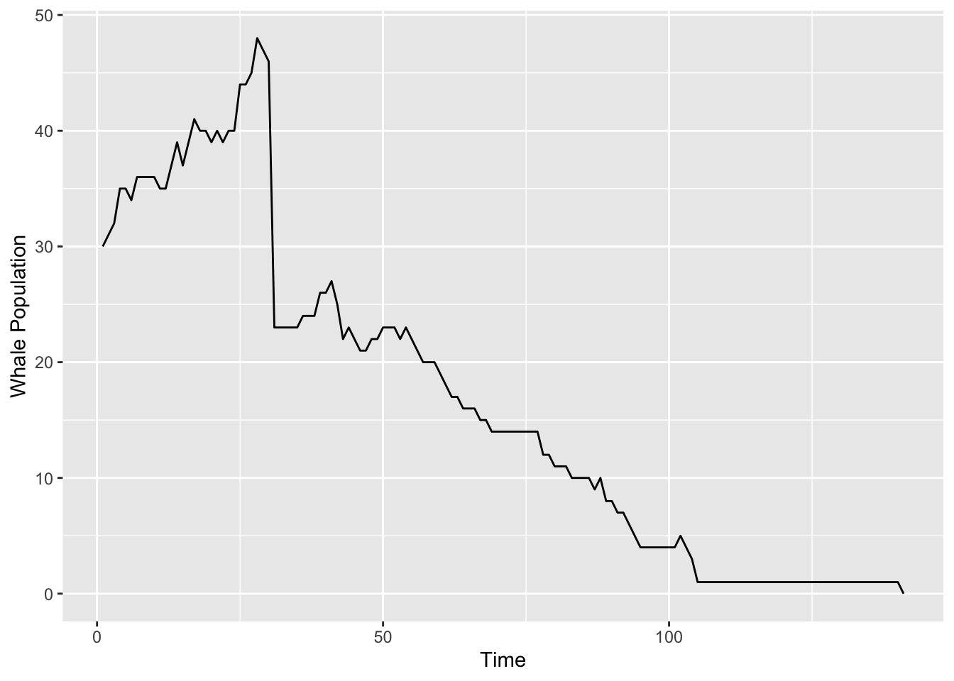
Figure 15.1: Simulated whale population. Sadly, they all die after about 130 days.

You should try running the simulation yourself a few times, for differing initial numbers of whales. If you like you can watch the whales move about by setting animate to TRUE:

oceanSim(
  steps = 200, males = 15, females = 15,
  animate = TRUE
)

You might also wish to explore varying the starve parameter: recall that the higher it is, the lower the long-term stable whale population will be. In order to better detect long-term stable population sizes, you will want to work with more steps, and you should turn off the step-by-step-animation, thus:

oceanSim(
  steps = 1000, males = 75, females = 75,
  starve = 2.5, animate = FALSE
)

The R package bcscr ((White 2023)) includes a more flexible version of the Ocean class that allows the users to set custom initial populations, including characteristics that vary from whale to whale.

The object-oriented approach to simulation is not necessarily the quickest approach: R6 objects do require a bit more time for computation, as compared to a system that stores relevant information about the population in vectors or in a data frame. On the other hand the object-oriented approach makes it easy to encode information about each individual whale as it proceeds through time. In larger applications, an object-oriented approach to programming can result in code that is relatively easy to read and to modify, albeit at some cost in terms of speed.

15.7 Generic-Function OO

We now turn to the second major type of object-oriented programming that is supported by R, namely: generic-function OO.

15.7.1 Motivating Examples

We begin by revisiting the task of printing to the console.

Recall that whenever we type the name of an object into the console and press Enter, R interprets the input as a call to the print() function. Consider, for example, printing some portion of m111survey from the bcscr package:

df <- bcscr::m111survey[1:5, c("height", "weight_feel")]

If we want to print df, then either of the following two statements accomplish the same thing:

print(df) ## explicit directive to print results to Console

##   height   weight_feel
## 1     76 1_underweight
## 2     74 2_about_right
## 3     64 2_about_right
## 4     62 1_underweight
## 5     72 1_underweight

df ## R implicity calls print() at top-level

##   height   weight_feel
## 1     76 1_underweight
## 2     74 2_about_right
## 3     64 2_about_right
## 4     62 1_underweight
## 5     72 1_underweight

Both expressions, as we learned long ago, involve a call to the print() function.

But let’s think a bit more deeply about what we see in the Console.

It is tempting to think of the above printouts as simply what the object df is. But that’s not quite right. In truth, it merely reflects how R represents df to us in the console. R was programmed to represent df in spreadsheet-format—with variables along columns, individuals along rows, and with handy row-numbers supplied—because human users are accustomed to viewing data tables in that way.

But now let us turn df into a list:

lst <- as.list(df)
str(lst)

## List of 2
##  $ height     : num [1:5] 76 74 64 62 72
##  $ weight_feel: Factor w/ 3 levels "1_underweight",..: 1 2 2 1 1

And let’s print lst:

lst # same as print(lst)

## $height
## [1] 76 74 64 62 72
## 
## $weight_feel
## [1] 1_underweight 2_about_right 2_about_right 1_underweight
## [5] 1_underweight
## Levels: 1_underweight 2_about_right 3_overweight

We get the familiar output for a list whose elements are named. Users don’t expect lists to be represented in the console in spreadsheet-style format, even if the elements of the list happen to be vectors that are all of the same length. They expect a more “neutral” representation, and R delivers one.

Printing to the console is a common task. It appears, however, that the method by which that task is performed depends on the type of object that is input to the print() function:

If your object is a data frame, print() behaves one way.
If your object is a list, print does something else.

Since the behavior of print() depends on the type of object involved in the operation of printing, you could say that it exhibits polymorphism. .

In fact it is the class of the object given to print() that determines the method that prints() employs. The class of an R-object can be accessed with the class() function :

class(df)

## [1] "data.frame"

class(lst)

## [1] "list"

How does the class of df determine the method used for printing? To see how this is done, look at the code for the print() function:

print

## function (x, ...) 
## UseMethod("print")
## <bytecode: 0x108da3d40>
## <environment: namespace:base>

The body of the print() consists of just one expression: UseMethod("print"). On the fact of it, this doesn’t seem to accomplish anything! In reality, though, a lot is taking place under the hood. Let’s examine what happens, step-by-step, when we call print(df).

The data frame df is assigned to the parameter x in the print() function.
We call UseMethod("print").
From help(UseMethod) we learn that UseMethod() takes two parameters:
- generic: a character string that names the task we want to perform. In this case generic has been set to “print”.
- object: this is an object whose class will determine the method that will be “dispatched”, i.e., the method that will be used to print the object to the console. By default this is the first argument in the enclosing function print(), so object gets set to the data frame df.
Control has now passed to the UseMethod() function, which searches for a suitable method for printing an object of class data.frame. It does this by pasting together “print” (the argument to generic) and data.frame (the class of the object df it was given) with a period in between, getting the string “print.data.frame”. A search is now conducted for a function having that name.

The function print.data.frame() will be found. We can tell because it appears on the list of available “methods” for print(). The methods() function will give us the complete list of available methods, if we like

methods("print")

## [1] print,ANY-method                                  
## [2] print,diagonalMatrix-method                       
## [3] print,sparseMatrix-method                         
## [4] print.abbrev*                                     
## [5] print.acf*
## ...
## [87] print.data.frame  <== Here it is!
## [88] print.data.table
## ...

R now calls the print.data.frame(), passing in df. The data frame is printed to the console.
When UseMethod() completes execution, it does not return control to the enclosing function print() from which it was called. The work of printing is done, so R arranges for control to be passed back to whomever called print() in the first place.

It is interesting to note that the very act of “printing out” the print function, which we did earlier in order to see the code for the function, involved a search for a printing method:

print # this is equivalent to print(print)

## function (x, ...) 
## UseMethod("print")
## <bytecode: 0x108da3d40>
## <environment: namespace:base>

In the call print(print), R looked at the class of print(), and found that it was of class function:

class(print)

## [1] "standardGeneric"
## attr(,"package")
## [1] "methods"

R then searched for a method called print.function and found one. Note that this method gives the sort of output to the console that would be helpful to a user:

the code for the function;
the location of the function in memory: 0x108da3d40;
the environment in which the function was defined (the package base).

Things go a little bit differently in the call to print(lst). The class of lst is list, but when you search the results of methods(print) you won’t find a print.list() method; accordingly R uses a fall-back method called print.default(). This is why the console-output for lists looks so “neutral.”

15.7.2 Terminology

The print() function is an example of a generic function. A generic function is simply a function that performs a common task by dispatching its input to a particular method-function that is selected on the basis of the class of the input to the generic function. Languages that use generic functions are said to support generic-function OO.

In message-oriented OO, objects own their own methods, and the way a task is performed depends on the class of the object that is invoked to perform the task. Generic-function OO, which is most commonly found in languages that support functional programming, puts more stress on functions: the generic function “owns” the methods in the sense that it acts as the central dispatcher, assigning a method function to perform a given task. In a bit of a reversal to message-passing OO, the method selected in generic-function OO depends on the class of the input-object to the generic, not on the class of the generic that was called to perform the task.

We should also mention that R actually has two ways to implement generic-function OO:

S3 classes;
S4 classes.

S3 classes were the first to be implemented, and to this day they are more commonly-used than S4 classes are. Therefore they are the implementation we will study. (S4 classes tend to be used by programmers in applications where there significant concern that the rules for formation of S3 classes aren’t strict enough.)

15.7.3 Common Generic Functions

There are three very commonly-used generic functions in R:

print(), which we have examined already;
summary();
plot().

Each of these generics is associated with a large number of method-functions. This is a great advantage to the casual user of R: one has to know only a few R-commands in order to acquire useful information about a wide variety of R-objects.

It is always a good idea to “try out” generic functions on objects you are using. You never know if the authors of R, or of a contributed package you have attached, may have written methods that are precisely tailored to that object.

Here are some example of the versatile, polymorphic behavior of the generic function summary():

heights <- df$height # vector of class "numeric"
summary(heights)

##    Min. 1st Qu.  Median    Mean 3rd Qu.    Max. 
##    62.0    64.0    72.0    69.6    74.0    76.0

feelings <- df$weight_feel # has class "factor"
summary(feelings)

## 1_underweight 2_about_right  3_overweight 
##             3             2             0

summary(df) # summarizing object of class "data.frame"

##      height            weight_feel
##  Min.   :62.0   1_underweight:3   
##  1st Qu.:64.0   2_about_right:2   
##  Median :72.0   3_overweight :0   
##  Mean   :69.6                     
##  3rd Qu.:74.0                     
##  Max.   :76.0

summary(lst)

##             Length Class  Mode   
## height      5      -none- numeric
## weight_feel 5      factor numeric

It is interesting also to see how R’s plot() (from package base) reacts to various types of input. See the Figure 15.2

x <- seq(-3, 3, by = 0.01)
plot(x^2)

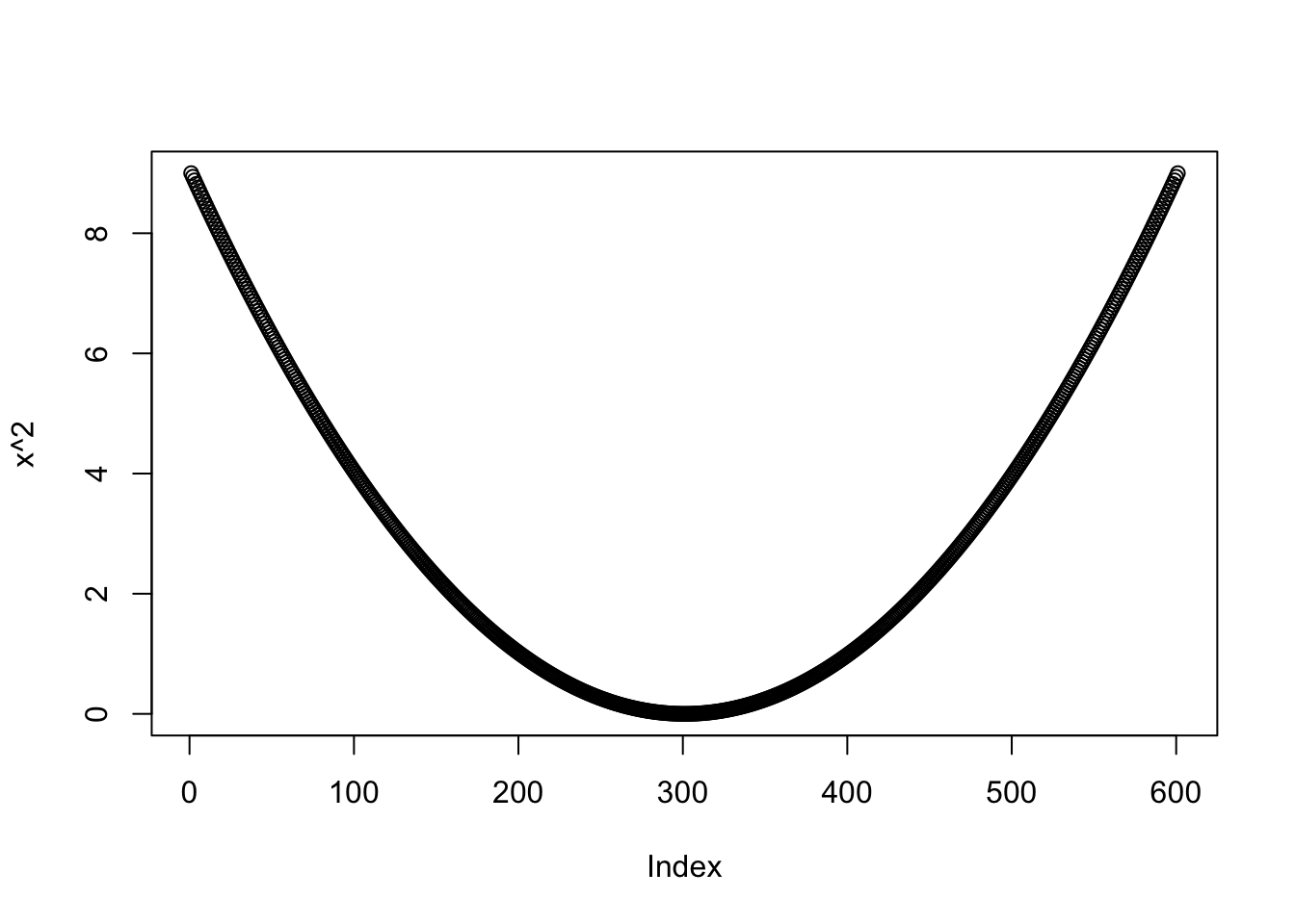
Figure 15.2: Our vector graphed as a parabola!

15.7.4 Writing Your Own Methods

As you advance in your programming skills, you will transition from writing programs to help you accomplish your own tasks to writing programs that help others—who are not as proficient in programming as you are—get some of their work done. Since casual users of R often become accustomed to generic functions as providers of useful information about many types of R-objects, you might find yourself writing methods for one or more of the common generic functions. In this Section will we will practice the art of method-writing: we will write some method-functions to report on the results of a simulation.

Recall the problem from Section 6.7 about estimating the expected number of uniform random numbers one must create until their sum exceeds a specified target-number. Let’s rewrite the simulation function so that it returns an object of a special class. We will then write print and plot methods that permit a user to obtain information about the results of any simulation that was performed.

First of all, let’s rewrite numberNeededSim():

numberNeededSim <- function(target = 1, reps = 1000,
                            seed = NULL) {

  # set the seed if none is provided
  if (!is.null(seed)) {
    set.seed(seed)
  }

  numberNeeded <- function(target) {
    mySum <- 0
    count <- 0
    while (mySum < target) {
      number <- runif(1)
      mySum <- mySum + number
      count <- count + 1
    }
    count
  }

  needed <- numeric(reps)
  for (i in 1:reps) {
    needed[i] <- numberNeeded(target)
  }
  results <- list(target = target, sims = needed)
  class(results) <- "numNeededSims"
  results
}

In the above code you will note that there is no longer a parameter table to permit printing of a table to the console. Also, nothing at all is cat-ed to the console. Instead we return only a list with two named elements:

target: the target you want your randomly-generated numbers to sum up to;
sims: the number of numbers required to sum to the target, in each repetition of the simulation.

The class of the returned list is set as “numNeededSims”.

Next, we write a print-method function. Its name must be print.numNeededSims. All of the table output and cat-ing to the console goes here:

print.numNeededSims <- function(x) {
  cat("The target was ", x$target, ".\n", sep = "")
  sims <- x$sims
  reps <- length(sims)
  cat("Here is a table of the results, based on ", reps,
    " simulations.\n\n",
    sep = ""
  )
  tab <- prop.table(table(sims))

  # for sake of pretty output,
  # remove "sims" variable name from top of table printout
  colNames <- dimnames(tab)
  names(colNames) <- NULL
  dimnames(tab) <- colNames

  print(tab)
  cat("\n")
  cat("The expected number needed is about ",
    mean(sims), ".\n",
    sep = ""
  )
}

Finally, let’s write a plot method. Its name must be plot.numNeededSims. This method will produce a bar graph of the results of the simulations. We’ll use the ggplot2 plotting package, so we should stop if the user hasn’t installed and attached ggplot2.

plot.numNeededSims <- function(x) {
  if (!"package:ggplot2" %in% search()) {
    return(cat("Need to load package ggplot2 in order to plot."))
  }

  sims <- x$sims
  # for a good bar-plot, convert numerical vector sims
  # to a factor with appropriate levels
  levels <- min(sims):max(sims)
  sims <- factor(sims, levels = levels)

  df <- data.frame(sims)
  plotTitle <- paste0("Results of ", length(sims), " Simulations")
  # in the code below, scale_x_discrete(drop = f) ensures that
  # even if there are no values in sims for a particular level it
  # will still appear in the plot as a zero-height bar
  ggplot(df, aes(x = sims)) + geom_bar() + scale_x_discrete(drop = FALSE) +
    labs(x = "Number Needed", title = plotTitle)
}

Let’s give it a try:

numberNeededSim(reps = 10000, seed = 4040)

## The target was 1.
## Here is a table of the results, based on 10000 simulations.
## 
##      2      3      4      5      6      7 
## 0.4974 0.3354 0.1253 0.0339 0.0068 0.0012 
## 
## The expected number needed is about 2.7209.

The print function was called implicitly, so we got useful output to the console.

It’s also possible to save the results somewhere, for example:

results <- numberNeededSim(reps = 10000, seed = 4040)
str(results)

## List of 2
##  $ target: num 1
##  $ sims  : num [1:10000] 3 2 2 2 3 3 4 2 2 5 ...
##  - attr(*, "class")= chr "numNeededSims"

Then it’s possible for the user to recall specific features of the results, for example:

results$target # get just the target number

## [1] 1

If we wanted the printout we could just say:

results

## The target was 1.
## Here is a table of the results, based on 10000 simulations.
## 
##      2      3      4      5      6      7 
## 0.4974 0.3354 0.1253 0.0339 0.0068 0.0012 
## 
## The expected number needed is about 2.7209.

For a plot we can use the plot() generic. The resulting graph appears as Figure 15.3.

plot(results)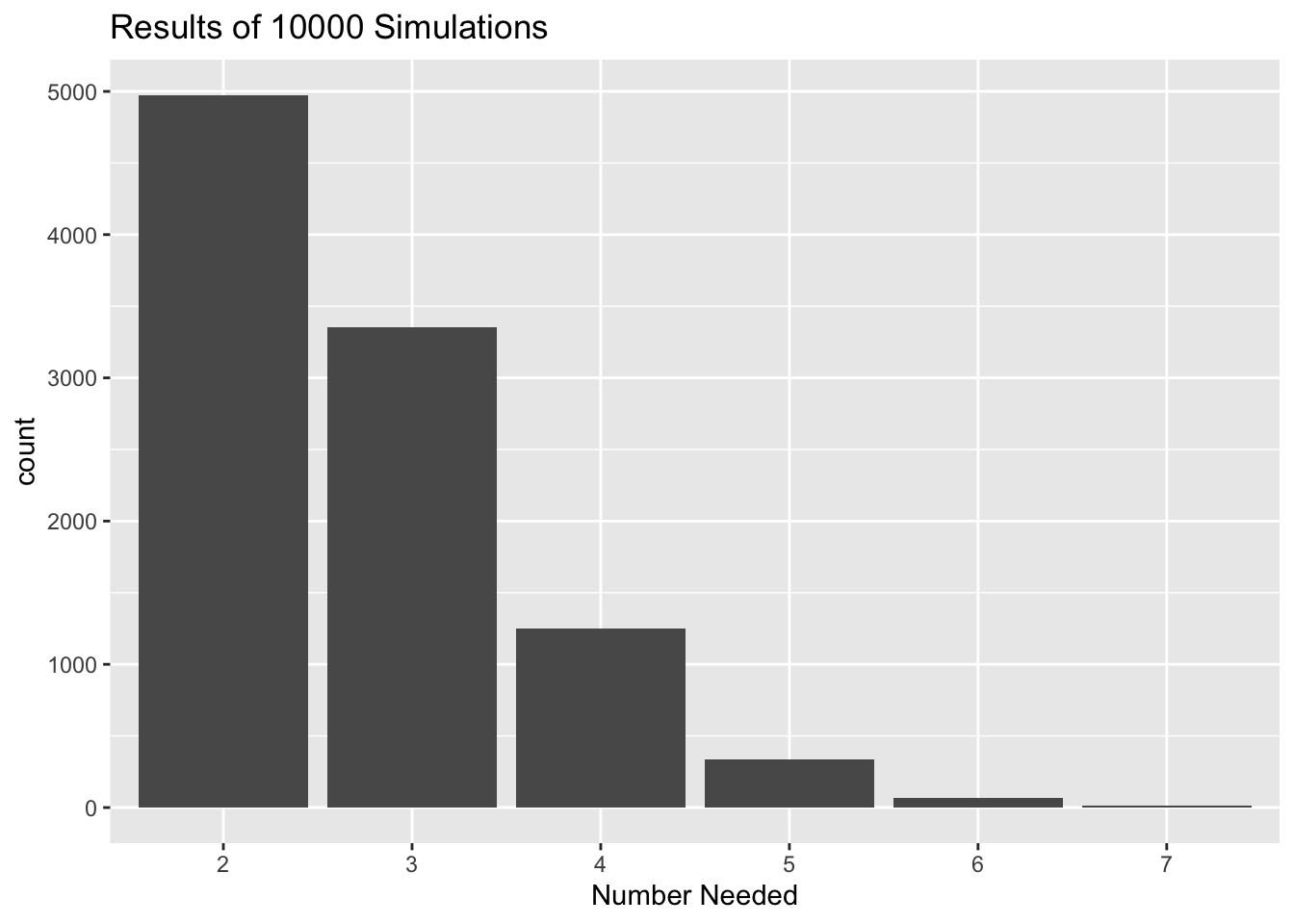

Figure 15.3: Results of the Number-Needed simulation.

15.7.5 Writing a Generic Function

Generic functions are most useful when they correspond to tasks that are so commonly performed that many methods are written for them, so that users get in the habit of “trying out” the generic on their object. As a consequence, the vast majority of method-functions are written for currently-existing, very well-known generics like print(), summary() and plot(). It doesn’t make a lot of sense to write generics that will have only a few methods attached to them. Nevertheless, it’s highly instructive to see how generics do their work, so as an example we’ll write a new generic, along with a couple of method functions.³⁷

First let’s create some objects with special classes. Here are two objects of class “cartesianPoint”. Our intention is that they correspond to points on the plane, represented with the standard $x$ and $y$ Cartesian coordinates.

point1 <- list(x = 3, y = 4)
class(point1) <- "cartesianPoint"
point2 <- list(x = 2, y = 5)
class(point2) <- "cartesianPoint"

It is also possible to represent a point on the plan with polar coordinates. The elements of a polar coordinates representation are:

$r$: a non-negative real number that gives the distance from the origin to the point;
$\theta$: the angle measure (in radians) between the positive $x$-axis and ray from the origin to the point.

point3 <- list(r = 2, theta = pi / 2)
point4 <- list(r = 1, theta = pi)
class(point3) <- "polarPoint"
class(point4) <- "polarPoint"

In the definition above, point3 is the point that lies at $\pi/2$ radians (90 degrees) counter-clockwise from the positive $x$-axis. That means that it lies along the positive $y$-axis. It is 2 units from the origin, so in Cartesian coordinates it would be written as $(0,2)$. Similarly, point4 would be written in Cartesian coordinates as $(-1,0)$, since it lies one unit from the origin along the negative $x$-axis.

Now let us suppose that we would like to find the $x$-coordinate of a point. For points of class cartesianPoint this is pretty simple:

point1$x # gives x-coordinate

## [1] 3

If the point is given in polar coordinates, we must convert it to Cartesian coordinates. You may recall the conversion formulas from a previous trigonometry class. To get $x$, use:

\[x = r\cos \theta.\] To get $y$, use: \[y = r\sin \theta.\] Thus, to find the $x$-coordinate for point3, work as follows:

point3$r * cos(point3$theta)

## [1] 1.224647e-16

The result is 0 (to a tiny bit of round-off error).

We now write a generic function xpos() for the $x$-coordinate:

xpos <- function(x) {
  UseMethod("xpos")
}

We need to write our method functions, one for each point class:

xpos.cartesianPoint <- function(point) {
  point$x
}

xpos.polarPoint <- function(point) {
  point$r * cos(point$theta)
}

Now we can feed points of either class into the generic xpos() function:

xpos(point2)

## [1] 2

xpos(point4)

## [1] -1

Glossary

Object-Oriented Programming: A programming paradigm in which programs are built around objects, which are complex structures that contain data.
Class: A general prototype from which individual objects may be created. The definition of the class specifies the attributes and methods that shall be possessed by any object created from that class. In addition, the definition of the class includes a function called an initializer that governs the creation of individual objects from the class.
Instantiation: The creation of an individual object as an instance of a class. The object gets all of the attributes and methods of the class (except for the initializer function). Typically the intializer functions allows for determination of the values of some of the object’s attributes at the time of instantiation.
Message-Passing OO: A type of object-oriented programming in which a task is performed by passing a message to the object that will perform the task. The method by which the object performs the task is determined solely by the class of which the object is an instance.
Attribute: A data-field belonging to an object that is not a function.
Method (also called “Method-Function”): A function that encapsulates a particular way of performing a task. In message-passing OO, it is a function data-field belonging to an object that as a data-field. Such a function usually has access to its inputs, to other data from its object, and to the objet itself. In generic-function OO, it is a function that is accessed through a generic function.
Reference Semantics: When an object has reference semantics, assignments involving that object create a pointer to the object, rather than creating a copy of the object itself.
Composition: The situation that arises when an object with reference semantics contains one or more other objects with reference semantics as data-fields.
Inheritance: The situation that arises when a class (known as the child class) is defined as being a particular type of some other class (known as the parent class). By default the child class has all of the attributes and methods of the parent class. The child class may be given additional attributes and methods.
Overriding: When a method defined in a child class has the same name as a method belonging to the parent class, then the child-class method is said to override the parent-class method. When the method is called on an instance of the child class the defining code in the child class, not the parent class, is used to execute the method.
Generic Function: A function that dispatches an input object to one of a number of method-functions, based on the class of the input.
Generic-Function OO: A type of object-oriented programming in which tasks are performed by generic functions. The method used to perform a particular task is determined by the class of the input object.
Polymorphism: A program exhibits polymorphism when a function behaves differently depending either on the type of object to which it belongs or the type of object to which it is applied.

Exercises

Write a new class called Witch that inherits from class Person. It should have two additional properties:
- slippers: Color of slippers worn by an individual witch. The initial value should be NULL.
- region: the part of Oz over which an individual witch reigns (e.g., “North”, “South”, etc.). The initial value should be NULL.
The class should include set-methods for both slippers and region. In addition there should be an initialize() method that overrides the method already provided with class Person. This new method should permit the user to set the value of slippers and region.

Create two new witches:
- The Wicked Witch of the East. Her name and desire are up to you, but her slippers should be silver, and of course she should reign over the East.
- Glinda, the Good Witch of the North. Her desire and color of slippers are up to you.
Attach the package bcscr, if you have not done so already:
```
library(bcscr)
```
Study the documentation for the classes Ocean, Female and Male, and then write your own ocean simulation in which the initial whales have properties that you select.

Run the simulation, initializing the ocean with ten whales of each sex and report on the results in an R Markdown document. (Note: Don’t run animations in an R Markdown document.)
Recall the function meetupSim() from Section 6.5, with which we investigated the probability that Anna and Raj would meet at the Coffee Shop. Suppose that we are interested not only in the probability that they meet, but also in the distribution of the number of minutes by which the latecomer misses the one who came early on the occasions when they do not manage to connect. Revise meetupSim() so that it does not print any results to the console, but instead returns a list. The list should have two elements:
- a logical vector indicating, for each repetition of the simulation, whether or not Anna and Raj met;
- a numerical vector indicating, for each repetition in which they did not meet, the number of minutes by which the latecomer missed meeting the person who arrived earlier.
Make the list have class “meetupSims”. A typical example of use should look like this:
```
results <- meetupSim(reps = 10000, seed = 3535)
str(results)
```
```
## List of 2
##  $ connect: logi [1:10000] FALSE FALSE TRUE FALSE TRUE FALSE ...
##  $ noMeet : num [1:6934] 30.275 29.959 22.394 0.491 4.898 ...
##  - attr(*, "class")= chr "meetupSims"
```
Building on the previous exercise, write a method-function called print.meetupSims() that prints the results of a meet-up simulation to the console. The function should provide a table that gives the proportion of times that Anna and Raj met, and a numerical summary of the simulation results when they did not meet. (You could use the summary() function for this.) A typical example of use would look like this:
```
results # has same effect as print(results)
```
```
## Here is a table of the results, based on 10000 simulations.
## 
## Did not connect       Connected 
##          0.6934          0.3066 
## 
## Summary of how many minutes they missed by:
## 
##     Min.  1st Qu.   Median     Mean  3rd Qu.     Max. 
##  0.00131  6.60680 14.55711 16.55834 24.87720 49.30534
```
Continuing in the same vein, write a method-function called plot.meetupSims() that makes a density plot showing the distribution of the number of minutes by which the latecomer misses the meeting. It should work like this:
```
plot(results)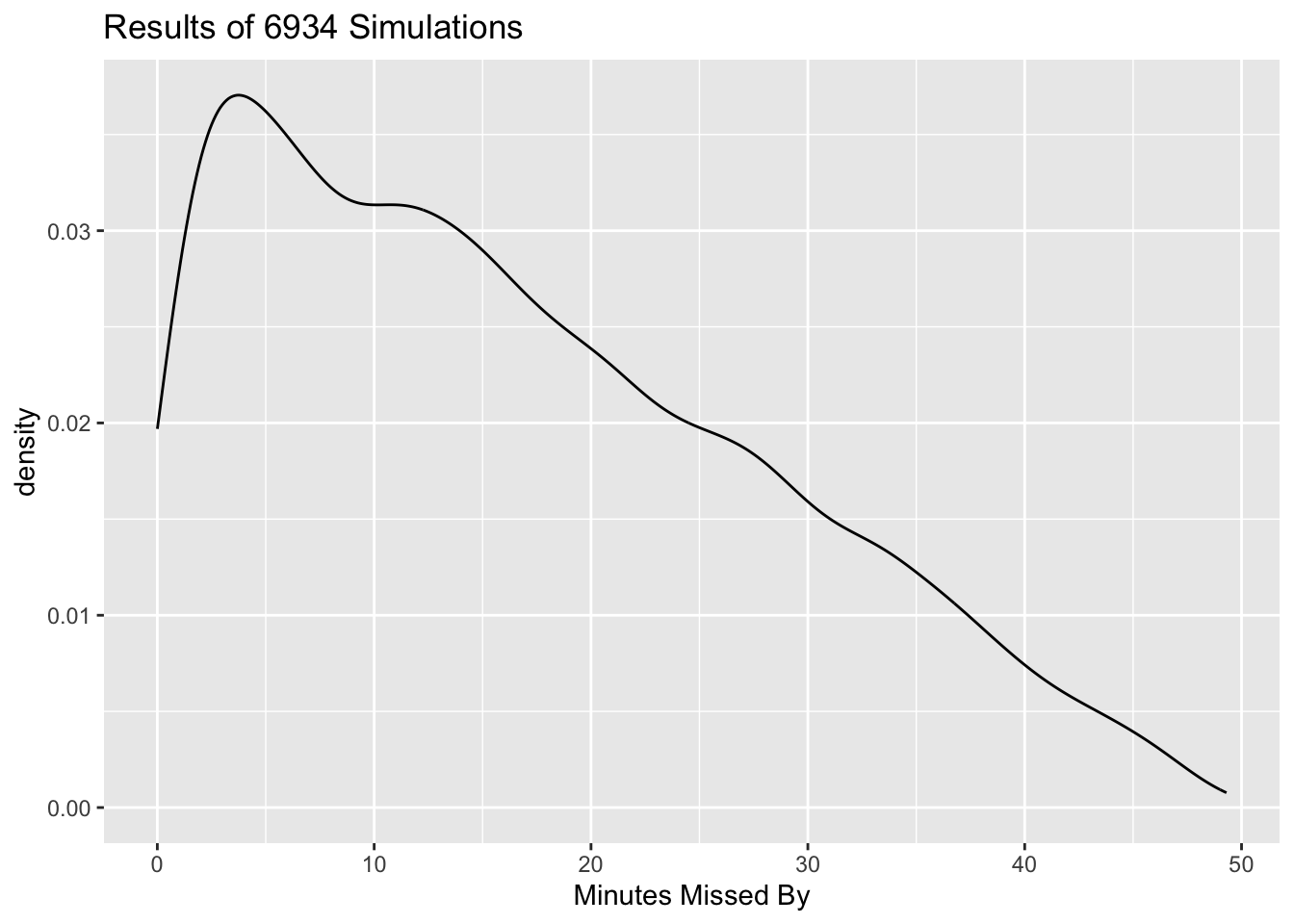
```
Write a generic function called ypos() that will return the $y$-coordinate of points of class cartesianPoint and polarPoint. Of course you will need to write the corresponding method functions, as well.
Write a generic function called norm() that will return the distance of a point from the origin. The point could be of class cartesianPoint or polarPoint, so you will need to write the corresponding method functions, as well. (It will be helpful to recall that for a point with Cartesian coordinates $(x,y)$ the distance from the origin is $\sqrt{x^2 + y^2}$.)

14 Functional Programming in R

16 Recursion