8 Graphics

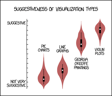
Figure 8.1: Violin Plots, by xkcd.

Now that we know a bit about how data can be stored and manipulated in data frames, we can begin to analyze data, so in this Chapter we will take a closer look at the aspect of data analysis known as data visualization. We’ll become acquainted with the grammar of graphics, a general approach to visualization, and then learn how this approach is implemented in the ggplot2 with which we have worked previously. Finally, we’ll engage in a case study.

8.1 The Grammar of Graphics

A graph begins with data, and the data we work with will be tidy data that comes in a data frame. Leland Wilkinson’s Grammar of Graphics (see (Wilkinson 2005)) posits that most quantitative graphics constructed from a data frame can be understood in terms of a few basic elements. In our quite elementary introduction to the Grammar, the elements to which we will pay the most attention are as follows:

Glyphs: the basic units of a graph. Glyphs represent cases in the data frame. Each glyph corresponds to one or more cases, but no two glyphs correspond to the same case.
Aesthetics: perceptual properties of glyphs that are not the same for all glyphs but instead vary depending on the values of variables for the case (or cases) that each glyph represents.
Frame: special aesthetics that relate the position of each glyphs in the graph to values of variables for the cases that the glyph represents.
Scales: particular choices that determine the precise relationship between aesthetic properties and data values for glyphs.
Guides: visual aids that help the human viewer to infer data values for cases from the aesthetic properties of the glyphs that represent them.

We will clarify these abstract ideas with a series of examples. Many of our examples will be drawn from the m111survey data frame in the tigerstats package.

library(bcscr)
help(m111survey)

You will recall that the data frame records the results of a survey of 71 students at Georgetown College in Kentucky. Each case (row in the frame) corresponds to an individual student. See Table 8.1.

Table 8.1: The first few rows of the m111survey data frame. Five variables are shown.
sex	fastest	GPA	seat	weight_feel
male	119	3.56	1_front	1_underweight
male	110	2.50	2_middle	2_about_right
female	85	3.80	2_middle	2_about_right
female	100	3.50	1_front	1_underweight
male	95	3.20	3_back	1_underweight
male	100	3.10	1_front	3_overweight

8.1.1 Example: a Scatterplot

We begin with a simple scatter plot based on the data. A scatter plot is often a good way to investigate graphically the relationship between two numerical variables. Figure 8.2 shows a scatter plot of student GPA vs. the fastest speed at which the student has ever driven a car.

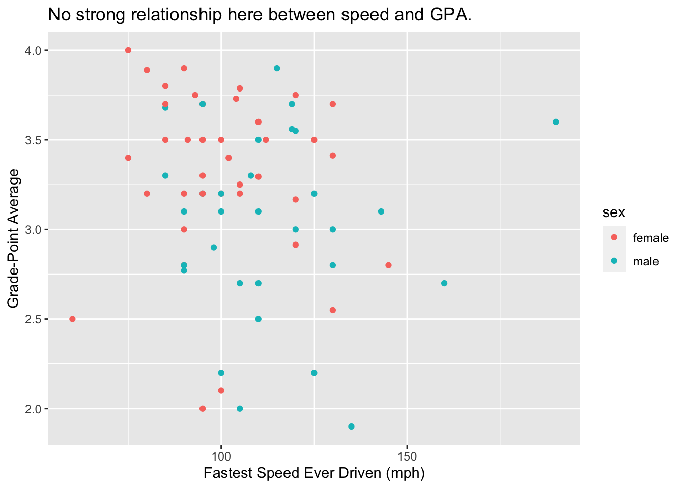
Figure 8.2: Scatterplot of fastest driving speed and GPA. Points are colored by sex of the student.

8.1.1.1 The Glyphs

In this scatter plot, the glyphs are points. Each case—each student in the survey—is represented by one and only one point on the plot.

8.1.1.2 The Aesthetics

In ordinary discourse the term aesthetic refers to any perceptual property of an object. For a point, the list of its perceptual properties includes its location, its shape, its size, its color, and so on. In the Grammar of Graphics, however, only some of the properties—the one that vary from glyph to glyph depending on data—count as aesthetics in the graph.

For the scatter plot, the property of size is not considered to be an aesthetic: we can see that this is so because all of the points are the same size, and so the size cannot vary with the values of some variable in the data frame. The same goes for the property of shape: all of the points in this scatter plot are circular.

On the other hand, the property of color IS an aesthetic for the glyphs in the graph, since the males and the females in the study are represented by points of different colors. You could say that color is mapped to the variable sex in the data frame:

the reddish color goes with the value “female”;
the turquoise color goes with the value “male”.

8.1.1.3 The Frame

In our scatter plot there are two other glyph properties that count as aesthetics:

x-location: the position of the glyph relative to the horizontal axis of the graph;
y-location: the position of the glyph relative to the vertical axis.

We can see that these properties are aesthetics because:

x-location is mapped to the variable fastest: the further to the right the glyph is, the greater is the value of fastest for the student represented by that glyph.
y-location is mapped to the variable GPA: the higher up the glyph is, the greater is the value of GPA for the student represented by that glyph.

Although x and y locations are just two more aesthetics, they are so crucial to the nature of a two-dimensional graph that they are classed separately in the Grammar of Graphics as the frame for the graph.

In the graphs we consider in this Chapter, the frame will always consist of at least the x-location, and sometimes—as in the case of our scatter plot—the y-location as well.

8.1.1.4 Scales

We can decide that color (for example) is to be mapped to sex, but that decision leaves open the question of how, precisely, to make the connection. The computer can make thousands of colors: which one will correspond to the value “male”, and which to “female”? To answer that question is to choose a scale.

In this example our scale was:

reddish = female
turquoise = male

But we might have adopted a different scale, such as:

blue = female
pink = male

Every aesthetic mapping involves a choice of a scale. Consider x-location: apparently a point on the extreme left of the scatter plot represent a student who drove 50 miles per hour. A point at the extreme right corresponds to a speed of 200 miles per hour, and in general the relationship between x-location and fastest is linear: for example, a point halfway across the graph goes with a speed of 125 miles per hour, halfway between 50 mph and 200 mph. In the same way, the mapping of y-location to GPA involves a linear choice of scale.

8.1.1.5 Guides

How were we able to see what the scales were for each of the three aesthetic mappings in the scatter plot? We were assisted by three set of guides, one for each mapping:

the legend to the right of the plot guided us from color to value of sex;
the labels and tick marks on the x-axis and the thin vertical white lines guided us from x-location to value of fastest;
the labels and tick marks on the y-axis and the thin horizontal white lines guided us from y-location to value of GPA.

Most of the time, every aesthetic mapping is accompanied by a guide that gives the human viewer at least a rough idea of the scale chosen for that mapping.

8.1.1.6 Summary

In summary we say that for this scatter plot:

The glyphs are points.
- This time each glyph represents one and only one case.
The frame is:
- x = fastest
- y = GPA
Other aesthetics are:
- color = sex
There are scales for the three aesthetic mappings above. (But we usually don’t say much about the x and y-location scales if they are linear, and we don’t make a big deal of the color scale unless we went to some trouble to choose it ourselves.)
The legend and the axis labels, tick marks and hash-lines are the guides.

8.1.2 Example: Two Bar Graphs

Bar graphs are useful in the study of categorical variables, especially factor variables that have only a few possible values. Figure 8.3 shows the distribution of the factor variable seat in the mat111survey data frame.

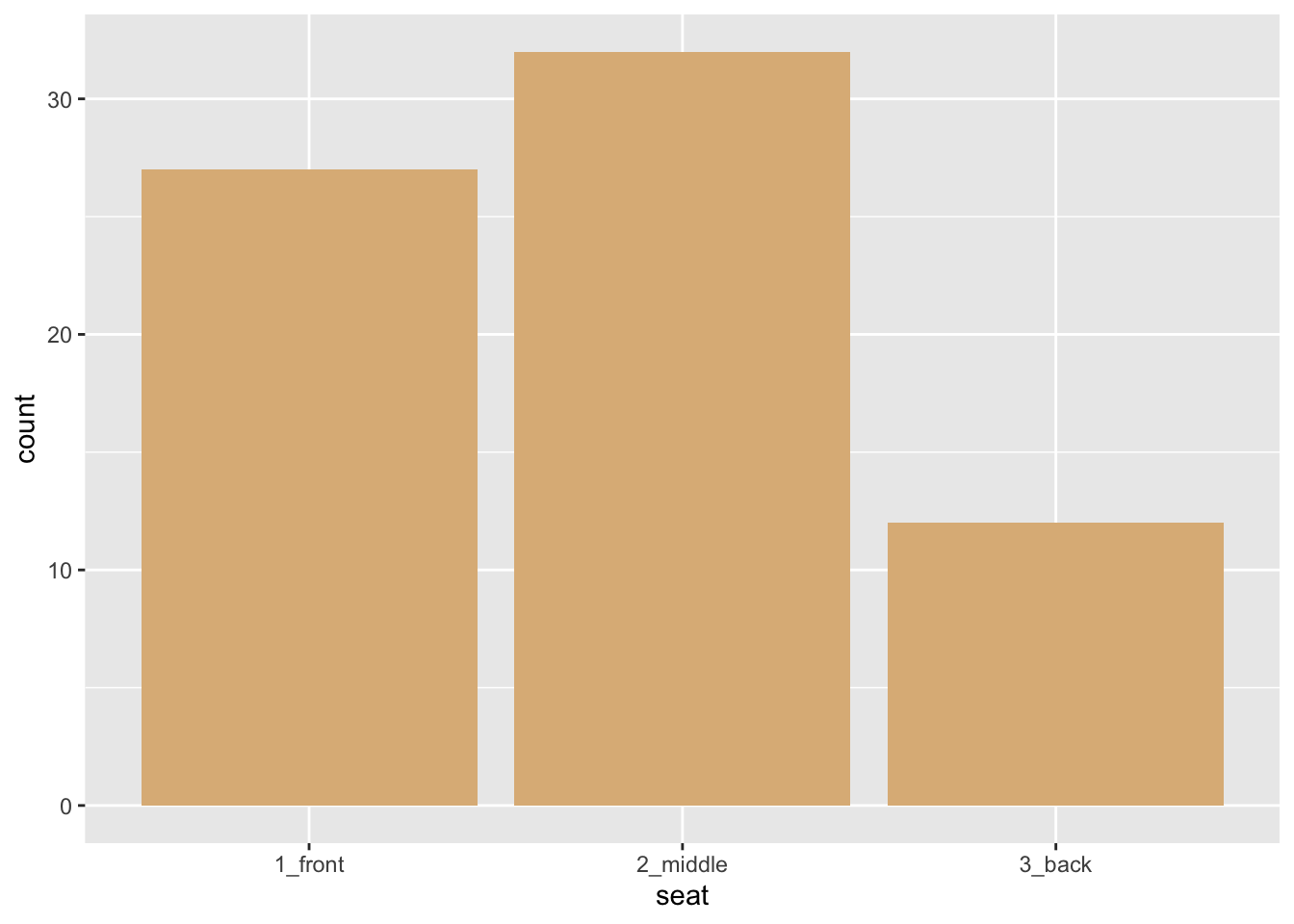
Figure 8.3: Bar graph of seating preference. The bars have a burlywood fill.

In this graph:

The glyphs are bars.
- This time each glyph an entire group of cases: there is a bar for the students who prefer the front, a bar for the students who prefer the middle, and a bar for the back-sitters.
The frame is:
- x = seat. Note that it is possible for x-location to map to a categorical variable!
- In this graph the y-location does not count as part of the frame, since it is not really an aesthetic. Instead the height of a bar along the y-axis tells us how many students are represented by that bar. In the Grammar of Graphics we say that the y-axis represents a statistic—a value computed from the data. In the situation at hand, our statistic is a simple tally of the cases for each value of seat.
There are no other aesthetics! The glyphs have various perceptual properties such as a shape rectangular and color, but these don’t vary with the cases: the shape is always rectangular and the color is always burlywood.
There is a scale for the x-location, but there is nothing very interesting about it: the three values of seat are equally spaced along the axis.
There is a guide for the x-location: labels on the x-axis tell us which bar goes with which value of the variable seat.

Bar graphs can also be used to study the relationship between two categorical variables. Figure 8.4 shows the relationship between sex and seating preference in the m111survey data.

Figure 8.4: Seating preference, by sex.

Again the glyphs are bars and each bar represents many cases, but now there is a bar for each combination of the values of sex and seat. The frame is again specified only by the x-location, but this time it is mapped to sex. There is another aesthetic as well: the color (more technically, the fill) of the bars is mapped to the variable seat, allowing us to see the relationship between the two categorical variables sex and seat. Scales and guides work much the same way as in the previous example.

8.1.3 Examples: Histograms, Density Plots and Box Plots

In this section we’ll examine some glyphs that are useful in the visualization of numerical variables.

8.1.3.1 Histograms

How are the fastest speeds driven distributed, for students in the m111survey data? In order to investigate such a question graphically, we might make a histogram like the one in Figure 8.5.

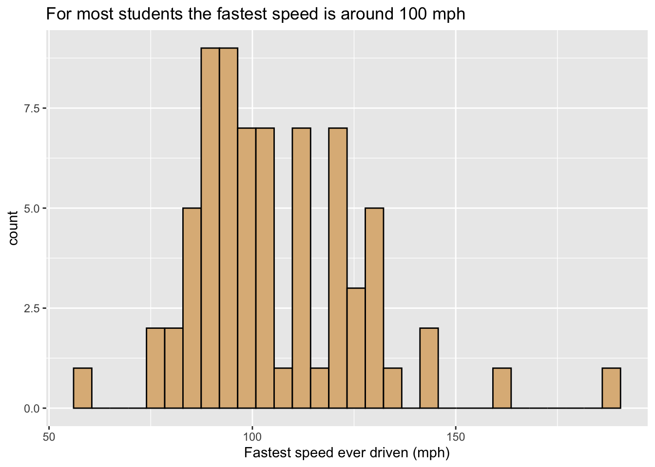
Figure 8.5: Histogram of the fastest speed ever driven.

In this graph:

The glyphs are rectangles. Each rectangle represents cases where the value of fastest lies within a particular range covered by the bottom left and right corners of the rectangle.
The frame is:
- x = fastest.
- As with our bar graphs, the y-location does not count as part of the frame, but instead represents a statistic, permitting the height of a rectangle to indicate the number of cases that it represents.
Again there are no other aesthetics. The burlywood fill of the rectangles is constant.
The scale for x-location, maps location to fastest in the familiar linear fashion, and the x-axis has the usual guides found for numerical variables.

Figure 8.6 is a variant, containing a second type of glyph: each student is now represented along the X-axis by a rug-tick located approximately at his or her fastest speed. (The ticks are actually “jittered” randomly so as to avoid over-plotting when two or more students report the same speed.) The addition of a second set of glyphs is called layering, and is a common device to enhance the communicative power of a graph.

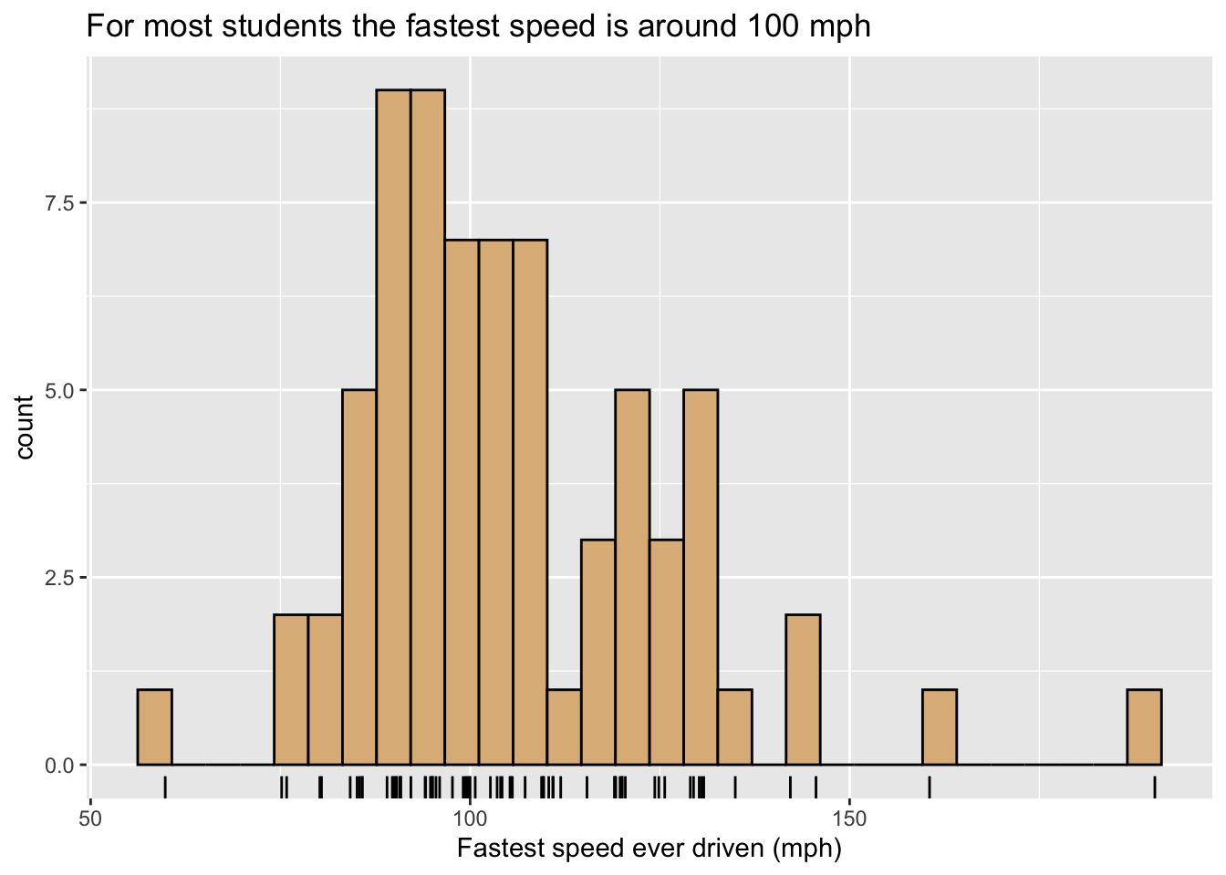
Figure 8.6: Histogram of the fastest speed ever driven.

8.1.3.2 Density Plots

One may also study the distribution of numerical variable with a density plot, as in Figure 8.7. In this figure there is only one glyph, the curve itself, and it represents all of the cases. However, its height represents crowding (density) of values of fastest for the cases: when the curve is high, many values are crowded closely together on the x-axis, and for speeds where the curve is low the viewer knows that few (if any) students drive around that speed. The y-axis is again used along with a statistic: for density plots the vertical scale is chosen in such a way that the total area under the density curve is 1, so that the area under the curve between two given speeds is approximately equal to the proportion of students who had speeds within that range. For density plots a rug, provided again by slightly jittered ticks, is a useful additional layer to indicate crowding of values.

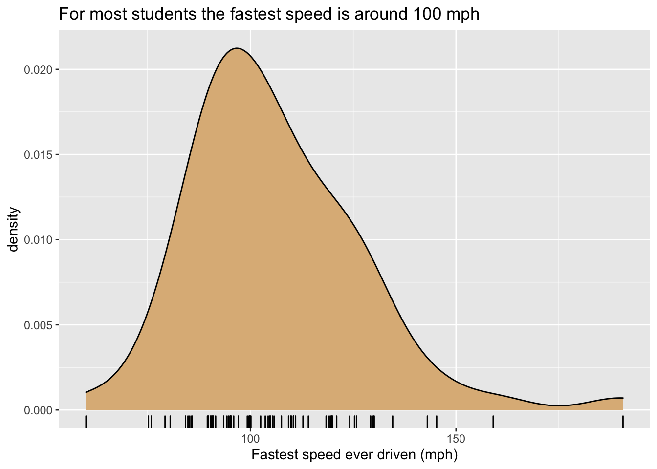
Figure 8.7: Density plot of the fastest speed ever driven.

Since they don’t take up much territory on a graph, density curves are especially useful when we want to study the relationship between a numerical and a categorical variable. For example, Figure 8.8 shows density plots of the fastest speeds for each of the three possible seating preferences. The glyphs are again density curves, but since the color aesthetic has been mapped to seat, we get a separate and differently-colored glyphs, one for each seating-preference..

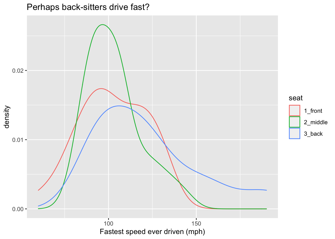
Figure 8.8: Density plot of the fastest speed ever driven.

Another approach to the same graphing problem is to use a type of glyph known as a violin. Look at Figure 8.9.

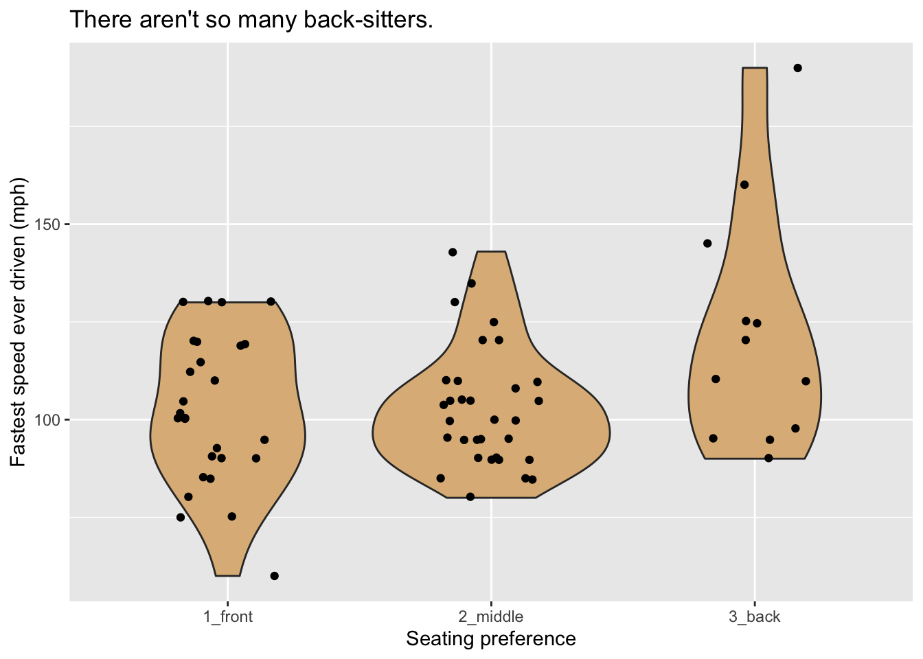
Figure 8.9: Violin plot of the fastest speed ever driven.

A violin glyph is simply two mirror-images of the same density plot, pasted together along their bases. Thus the violin is thick where many values are clustered together and thin where data values are rare. In this plot, the frame is constituted by mapping x-location to seat and y-location to the variable fastest. For additional communicative power we have layered another set of glyphs–jittered points, one for each case–onto the plot.

Suppose that one wished to incorporate a third variable, such as sex, into the graph? One possible way to to this is to divide the graphs into separate plots based on the values of one of the categorical variables in question. The separate plots are known as facets, and are illustrated in Figure 8.10, where facet-ing has been done on the basis of the variable seat.

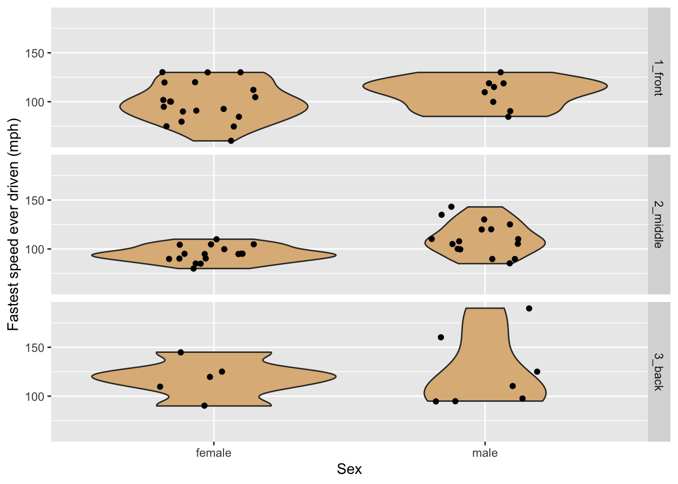
Figure 8.10: Violin plots of the fastest speed ever driven, by sex and seating preference.

8.1.3.3 Box Plots

The five number summary is a convenient way to summarize the distribution of a numerical variable. The five numbers involved are:

the minimum value
the first quartile $Q1$, the $25^{\text{th}}$ percentile of the values
the median, which is the $50^{\text{th}}$ percentile
the third quartile $Q3$, the $75^{\text{th}}$ percentile
the maximum value

Also of interest is the interquartile range $IQR$, defined as:

\[IQR = Q3 - Q1.\]

The interquartile range covers measures the spread in the middle 50% of the values.

In R the five number summary can be got quickly with the fivenum() function:

fnFastest <- fivenum(m111survey$fastest)
names(fnFastest) <- c("min", "Q1", "median", "Q3", "max")
fnFastest

##    min     Q1 median     Q3    max 
##   60.0   90.5  102.0  119.5  190.0

A box-plot glyph is the graphical counterpart of the five number summary. Figure 8.11 shows how it works for the variable fastest in the m111survey data frame. The box ranges from $Q1$ to $Q3$, covering the middle half of the speeds. The lower hinge extends from $Q1$ down to the minimum speed. The upper hinge would have extended from $Q3$ to the maximum value, but the maximum value was flagged as an outlier. When ggplot2 makes a box-plot, any point that is

greater than $Q3 + 1.5 \times IQR$ or
less than $Q1 - 1.5 \times IQR$

is flagged for individual plotting, and the corresponding hinge will be $1.5 \times IQR$ units long.

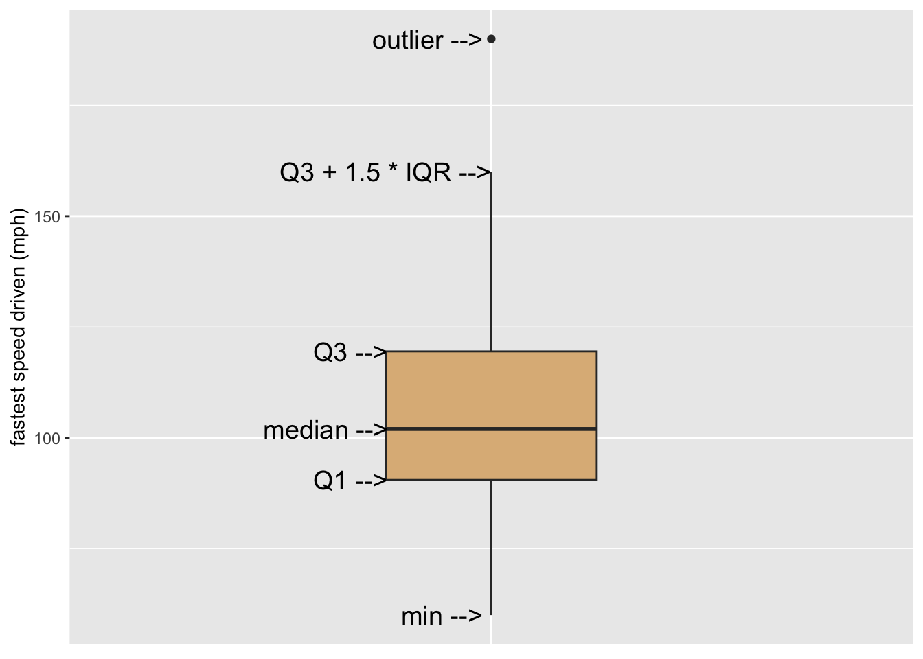
Figure 8.11: Illustration of a simple box plot.

A single box glyph on its own is not very interesting. Where box plots shine is in the study of the relationship between a numerical variable and a categorical with a large number of levels, as in Figure 8.12. Here the glyphs are boxes, with each box being constructed from the bills that were issued in a particular month.

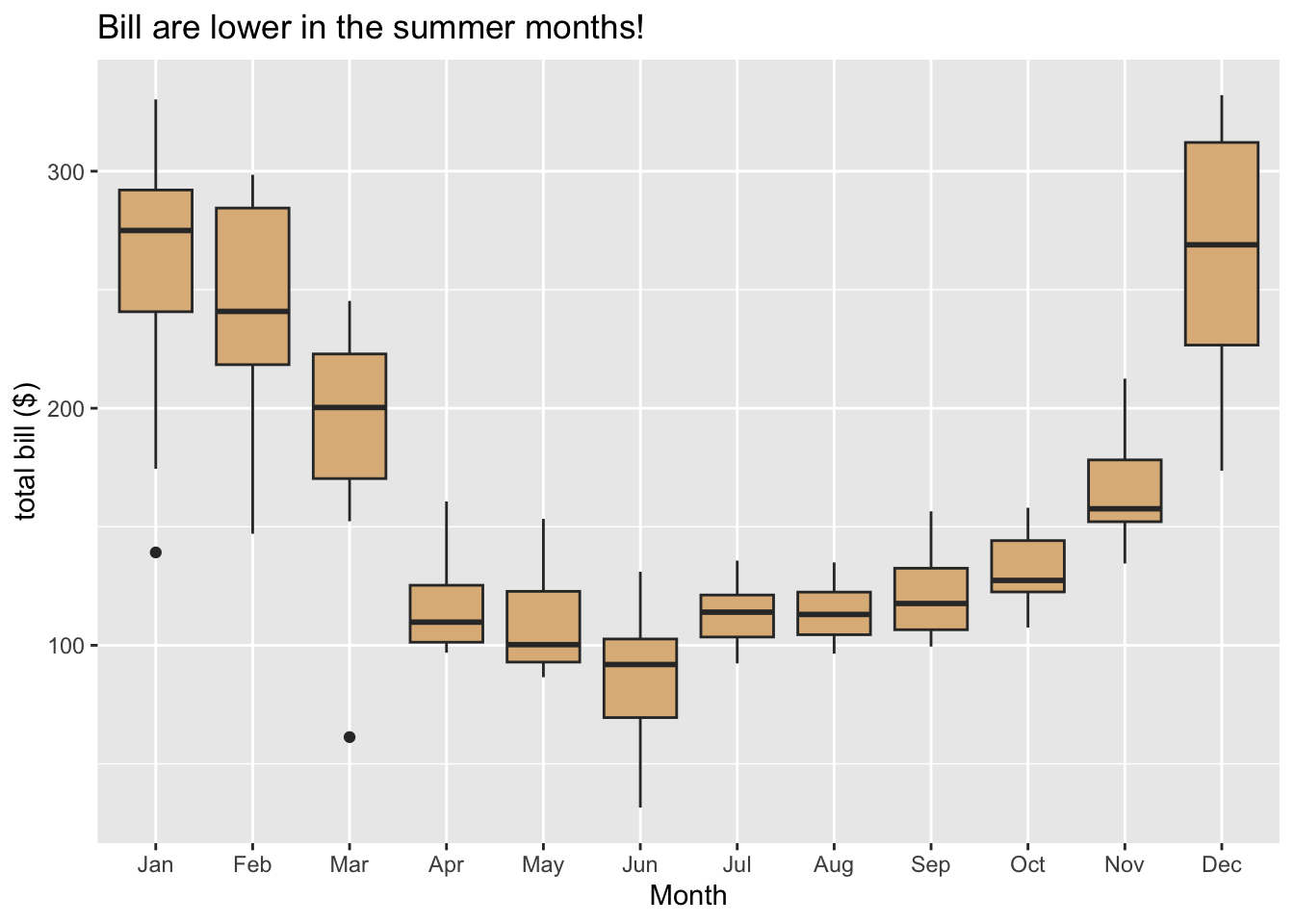
Figure 8.12: Utility bills through the year.

8.1.4 Example: Choropleth Maps

The term “choropleth” derives from Greek and means “many regions.” A choropleth graph is a graph in which the frame is provided by some sort of map with regions that might be countries, cities or counties in the U.S. etc.

In the choropleth map shown in Figure 8.13, is based on a data frame in which ease case is a state in the U.S (along with the District of Columbia). One of the variables is population, the population of the state. The glyphs are the territories of each of the U.S. states. The frame is determined by mapping x and y-location to latitude and longitude. The aesthetic property color is mapped to the population, and a guide is provided to the right of the graph.

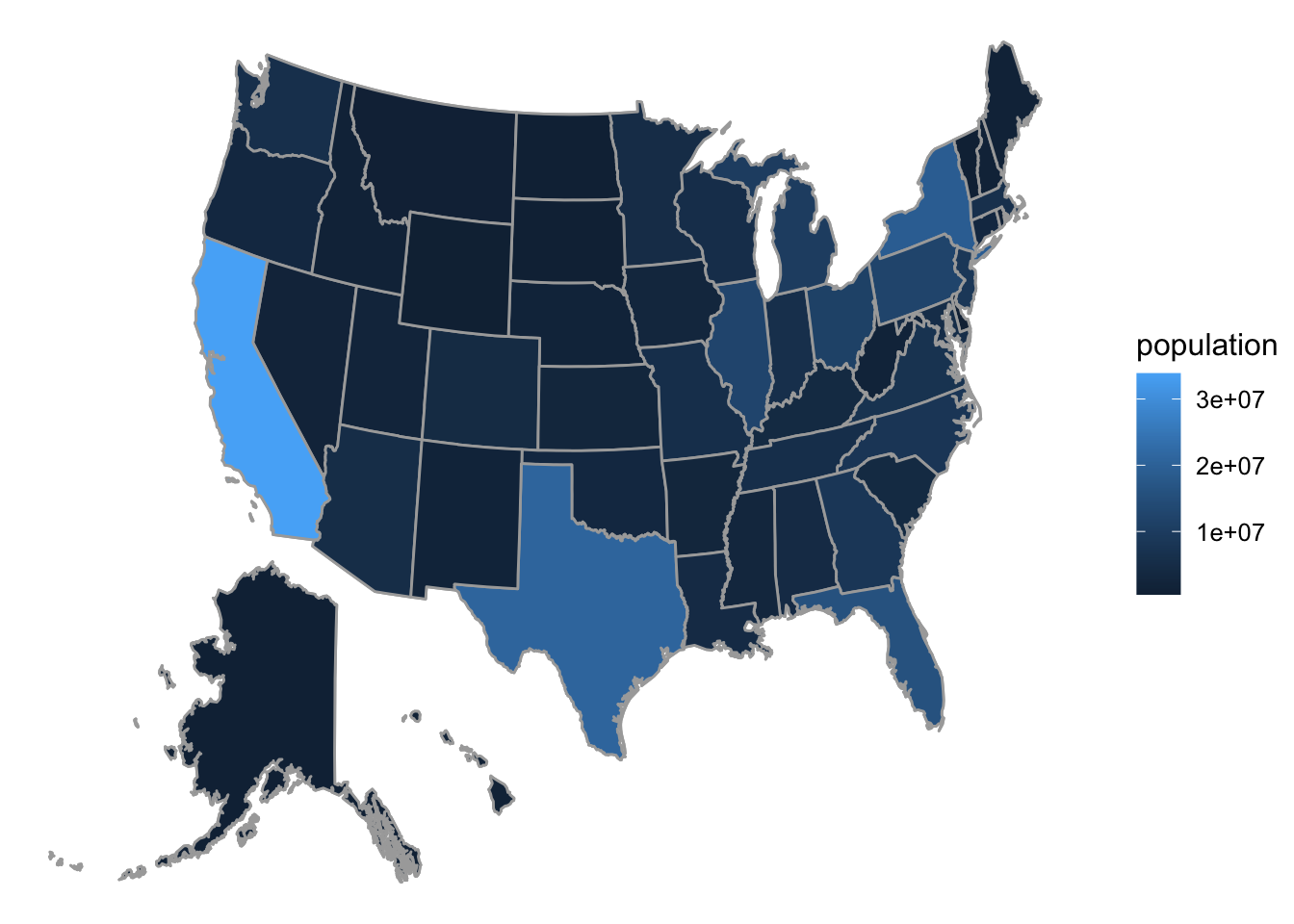
Figure 8.13: Choropleth map of state populations in the U.S.

8.1.5 Practice Exercises

In each of the exercises below, consult the Help for the relevant data frame. (You’ll need to identify variables by their names in the data frame when you discuss aesthetic mappings.)

The following graph is based on the data frame mosaicData::SwimRecords: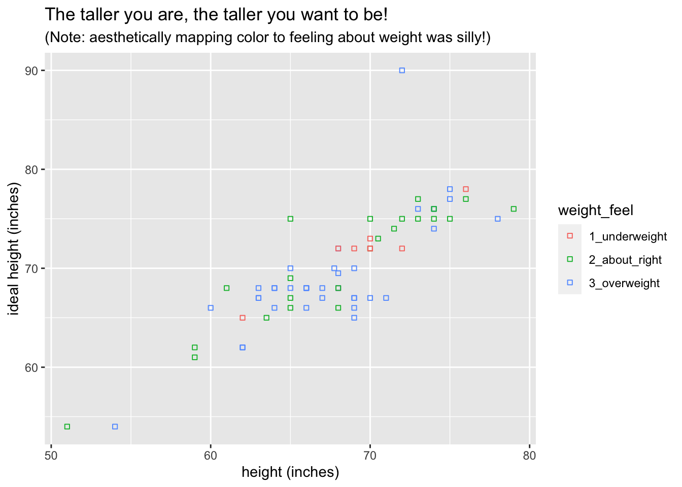
- What variables are used to make the frame?
- What are the two types of glyphs?
- What other aesthetic(s) are there (besides the x and y-locations in the frame)? To what variable(s) are they mapped?
- What guides do you see?
The following graph is based on the data frame mosaicData::KidsFeet:
- What variable(s) are used to make the frame?
- What are the two types of glyphs?
- What other aesthetic(s) are there (besides the frame)? To what variable(s) are they mapped?
- What guides do you see?
The following graph is based on the data frame mosaicData::Galton:
- What variable(s) are used to make the frame?
- What are the two types of glyphs?
- What other aesthetic(s) are there (besides the frame)? To what variable(s) are they mapped?
- What guides do you see?

8.1.6 Solutions to Practice Exercises

Answers:
- Frame: x -> year, y -> time;
- Glyphs: points and line-segments between pairs of points;
- Other aesthetics: point-color and line-color are both mapped to sex;
- Guides: legend for sex, axis labels and ticks for year and time.
Answers:
- Frame: x -> biggerfoot;
- Glyphs: bars;
- Other aesthetics: bar fill -> sex;
- Guides: legend for sex, axis labels and ticks for biggerfoot.
Answers:
- Frame: x -> father;
- Glyphs: density curve, jittered rug-ticks;
- Other aesthetics: none;
- Guides: axis labels and ticks for father.

8.2 Implementation in ggplot2

In its syntax, the ggplot2 package attempts to follow the Grammar of Graphics fairly closely. Let’s see how this works by building up, in step-by-step fashion, to our initial graph example—the scatter plot in Figure 8.2.

8.2.1 Basic Setup: the Data Frame

Construction of a graph in ggplot2 begins with the ggplot() function. The first parameter of the function is data, the value of which will be the data frame on which we plan to build the graph.

It is possible call ggplot() with just the data, and indeed it is instructive to do so. The result is seen in Figure 8.14: it is simply a blank window.

ggplot(data = m111survey)

Figure 8.14: A completely blank plot!

8.2.2 More Setup: Establishing the Frame

ggplot() has a second parameter, the parameter mapping. Usually it is assigned the result of a call to the ggplot function aes(), which is used to establish aesthetic mappings. The common procedure is to use this first call to aes() to establish the frame: later calls will map other aesthetics properties to other variables, as desired.

If we want to work toward Figure 8.2, we will have to map x-location to fastest and y-location to GPA. This is accomplished by the following code:

ggplot(data = m111survey,
       mapping = aes(x = fastest, y = GPA))

Figure 8.15: Just the frame: no glyphs yet!

The result appears as Figure 8.15. A frame has been established, along with guides to ggplot2’s default choice of linear scales for the mappings to fastest and to GPA.

It is worth noting that most programmers do not bother to name the data and mapping parameters. Figure 8.15 could just as well have been produced as follows:

ggplot(m111survey, aes(x = fastest, y = GPA))

In the future we will also drop these parameter names.

8.2.3 Labels

At any point we can add labels to our plot. If you are simply exploring data you don’t need labels, but if you are writing up the final version of a report you will want to give careful consideration to labeling axes and to providing a good title (or—if you are able to to do so—a good caption). The following code adds labels for the x and y axes, a title—and even a subtitle, although subtitles are somewhat rare in practice.

ggplot(m111survey, aes(x = fastest, y = GPA)) +
  labs(x = "fastest speed ever driven (mph)",
       y = "grade point average",
       title = "Dunno what to say, yet!",
       subtitle = paste0('A title should briefly indicate the main',
                         ' lesson the plot has for us.  Instead of:',
                         ' "Scatterplot of\nGPA vs. fastest speed",',
                         ' say something like: "Speed and GPA are',
                         ' not strongly related."'))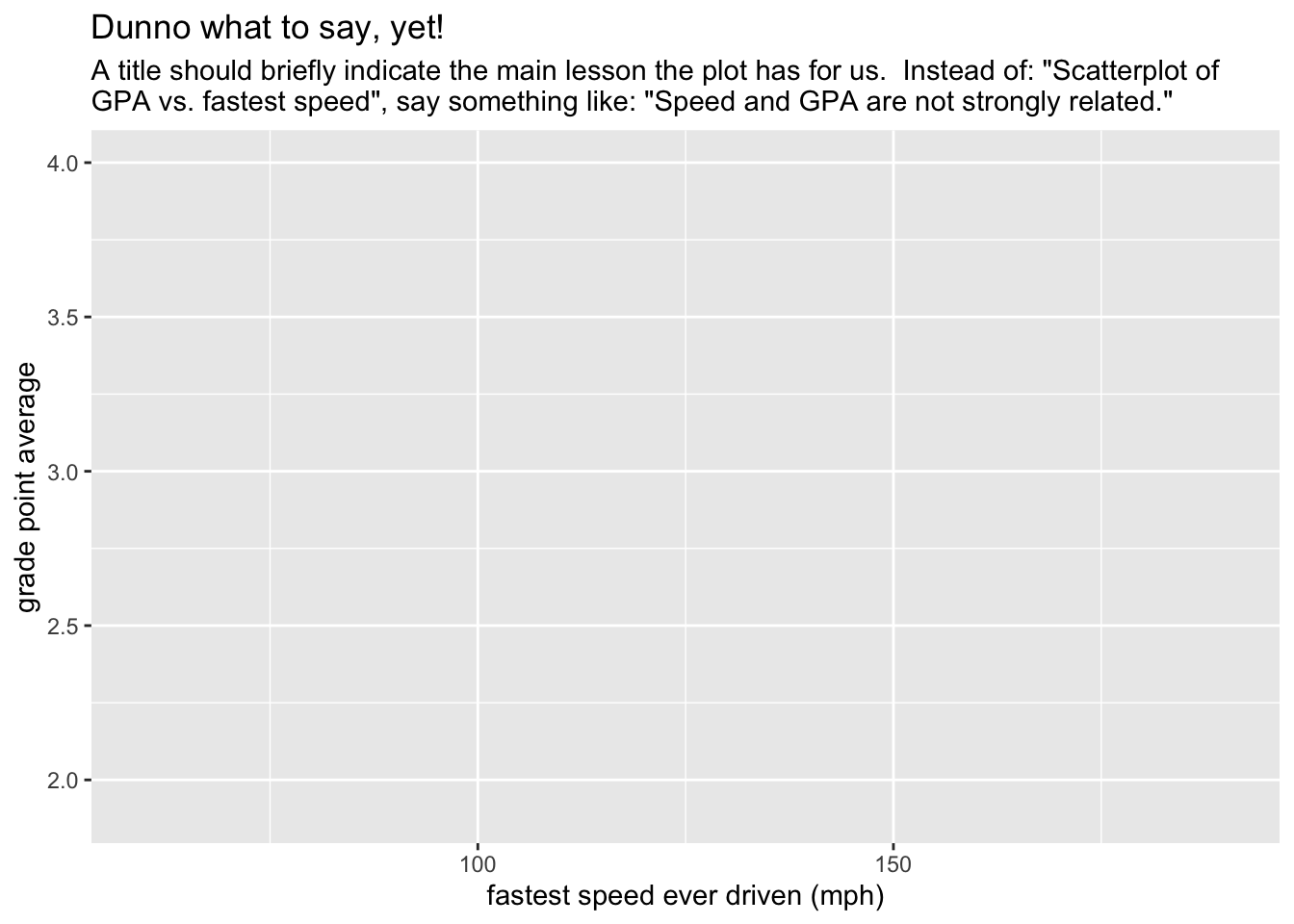

Figure 8.16: You can always add some labels!

8.2.4 Adding a Type of Glyph

It is high time now to make some data appear on our plot, so let’s add some glyphs. In ggplot2 syntax glyphs are added with functions whose names are of the form:

geom_gylphType()

Thus we have such things as:

geom_point() for points;
geom_line() for line segments between points;
geom_bar() for the bars of a bar graph;
geom_histogram() for the rectangles that make up a histogram;
geom_density() for the curve of a density plot;
geom_violin() for the violins of a violin plot;
geom_jitter() for jittered points representing individual cases;
geom_rug() for rug-ticks representing individual cases;
and a number of other geom’s!

8.2.4.1 Our First Geoms

Let’s add some points to the plot with the following code. The result appears as Figure 8.17. We are now quite close to the target plot.

ggplot(m111survey, aes(x = fastest, y = GPA)) +
  geom_point() +
  labs(x = "fastest speed ever driven (mph)",
       y = "grade point average",
       title = "Speed and GPA are not strongly related.")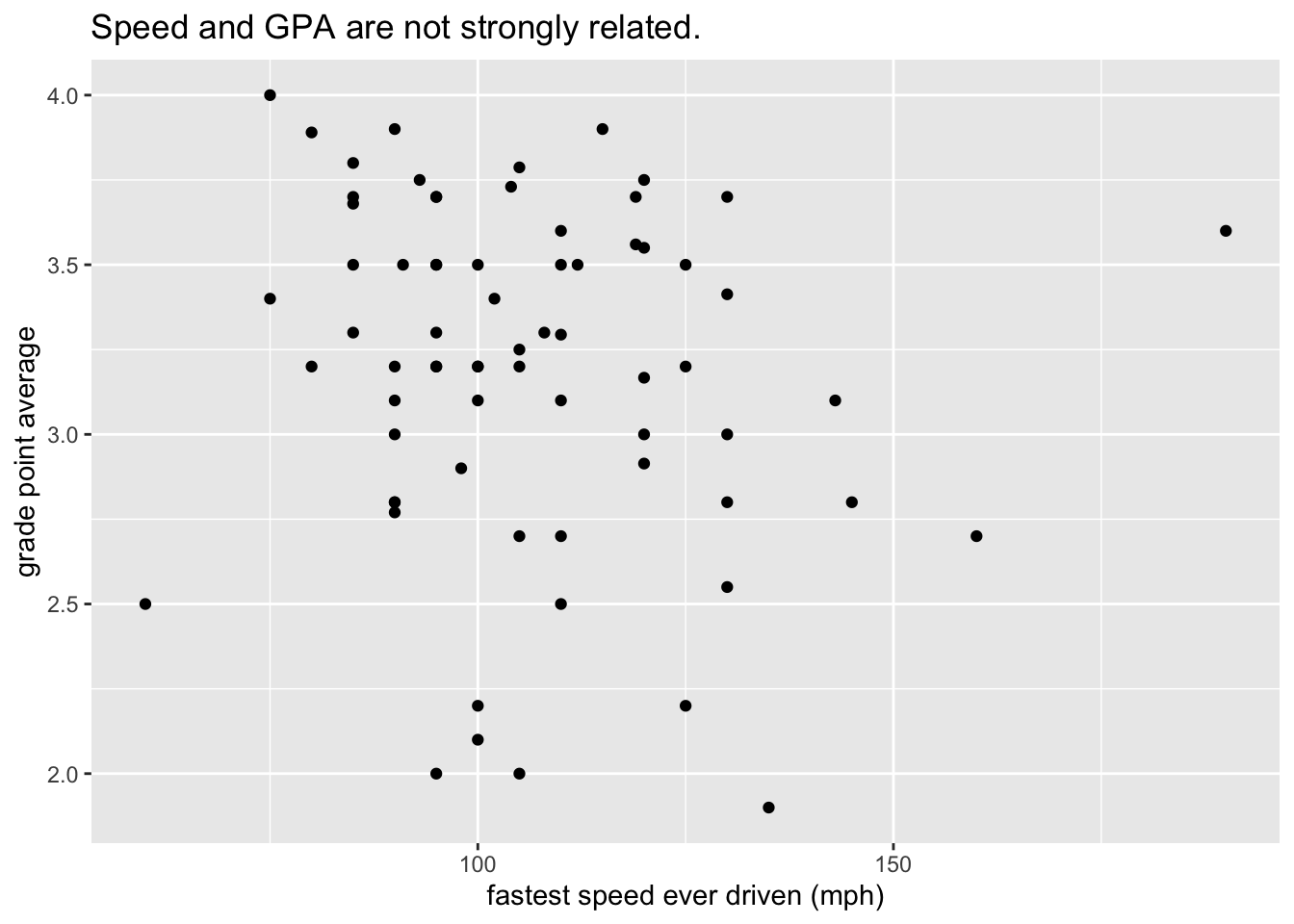

Figure 8.17: Finally: the data appears!

8.2.4.2 Further Aesthetic Mappings

The final step in our first example is to map the color property of points to the variable sex. We do so by a call to aes(). Conventionally a mapping for a glyph is accomplished inside the geom-function that creates the glyph, as in the code below that creates figure 8.18, our target plot:

ggplot(m111survey, aes(x = fastest, y = GPA)) +
  geom_point(aes(color = sex)) +
  labs(x = "fastest speed ever driven (mph)",
       y = "grade point average",
       title = "Speed and GPA are not strongly related.",
       subtitle = "(But guys tend to drive faster, and to have lower GPAs.)")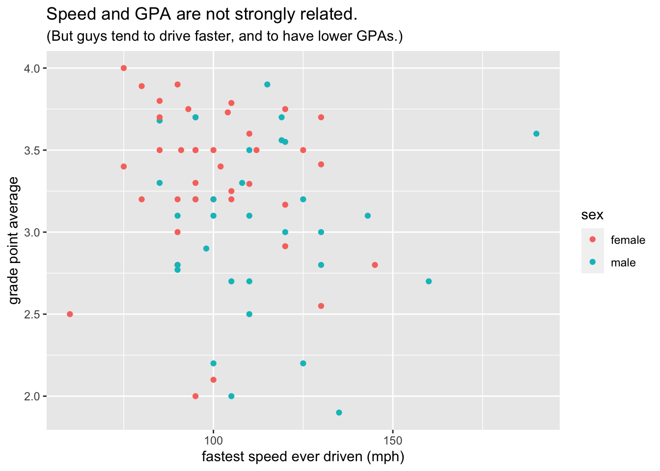

Figure 8.18: This is the target plot!

Points have other perceptual properties in besides their color. Shape is such a property. (From the point of view of the Grammar of Graphics, a point in itself is only an abstract location in space. Only when it assumes all of its perceptual properties does it actually “appear”, and when it does appear its shape may be other than circular, just as its color may be other than, for instance, black.) Thus alternative way to incorporate sex into the graph would have been to map shape to sex,as in the following code that results in Figure 8.19:

ggplot(m111survey, aes(x = fastest, y = GPA)) +
  geom_point(aes(shape = sex)) +
  labs(x = "fastest speed ever driven (mph)",
       y = "grade point average",
       title = "Speed and GPA are not strongly related.",
       subtitle = "(But guys tend to drive faster, and to have lower GPAs.)")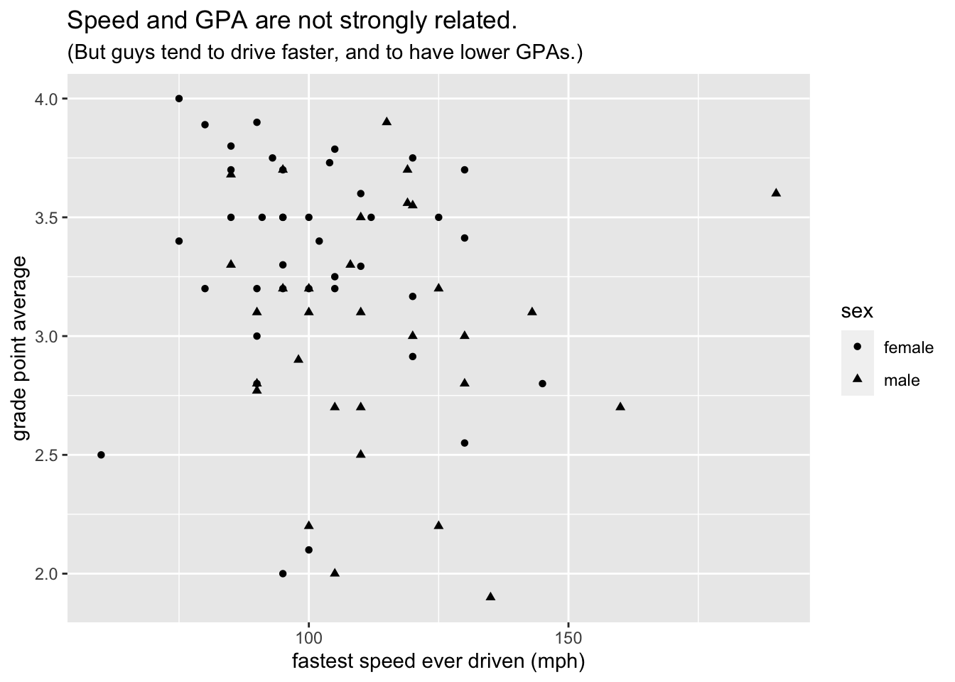

Figure 8.19: Mapping shape to the variable sex.

Passing now from our scatter plot example, we consider how to achieve another of the plots studied in the previous section, namely Figure 8.4. Following the same logic of calls to ggplot() and a geom-function, we see that the bar graph on sex and seating preference can be obtained by mapping the fill property of bars to seat as seen in the following code (results shown again as Figure `8.20)

ggplot(m111survey, aes(x = sex)) + 
  geom_bar(aes(fill = seat)) +
  labs(x = "Sex",
       title = "Males are more likely to prefer the Back!")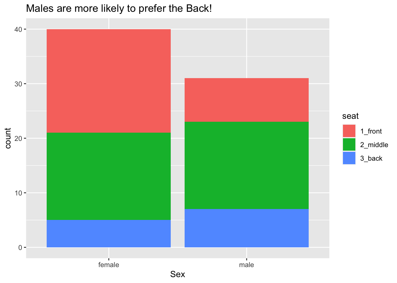

Figure 8.20: Seating preference, by sex.

Some people don’t like the glyphs “stacked” in bar graphs. In order to mollify them we can set position to “dodge”, as in the code below. The results appear in Figure 8.21.

ggplot(m111survey, aes(x = sex)) + 
  geom_bar(aes(fill = seat), position ="dodge")

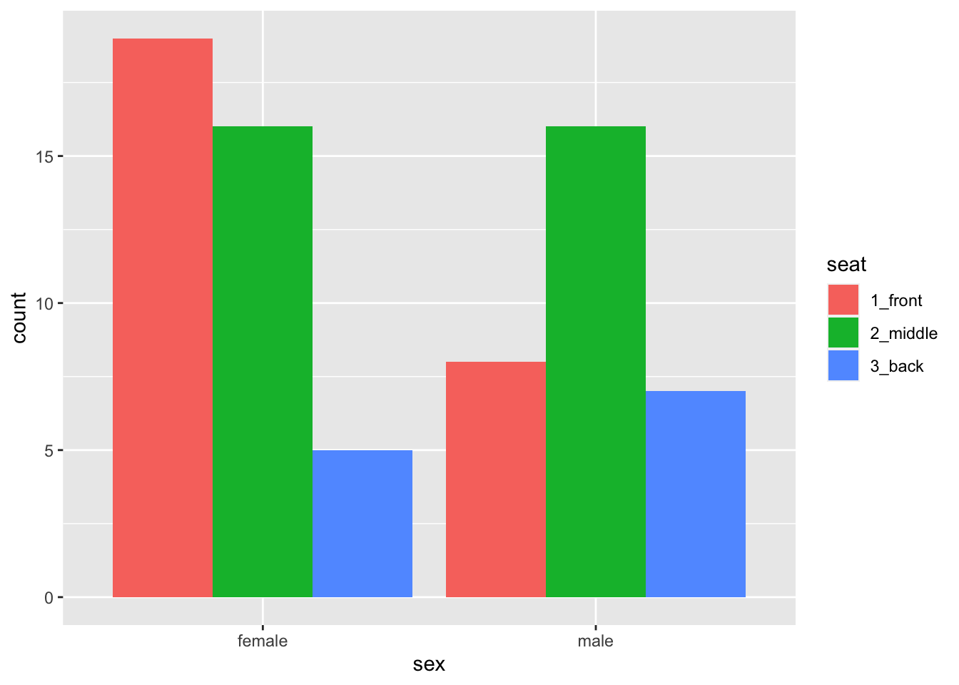
Figure 8.21: Seating preference, by sex—no stacking of bars..

Note that position is not an aesthetic property: all of the bar dodge each other. Dodgy-ness is not something that varies from glyph to glyph according to values in the data.

8.2.4.3 Aesthetic Mappings vs. Fixed Properties

It is wise to dwell a bit on the distinction between aesthetic mappings on the one and hand and fixed properties of glyphs on the other hand.

The key is this:

An aesthetic mapping are always accomplished as an argument in a call to aes(). In this argument, the aesthetic property is the parameter name, and a variable is assigned to it, thus:
- geom_bar(aes(fill = seat))
- geom_point(aes(color = sex))

A fixed property is determined by an argument to a geom-function call. The property to be fixed is the name of the parameter, and its constant value is the value supplied, thus:

Code	Effect
`geom_point(color = "blue")`	all the points are blue
`geom_point(shape = 22)`	all points are solid squares
`geom_point(size = 3)`	all points are bigger than default size(1)
`geom_bar(fill = "burlywood")`	all bars have the burlywood fill-color

As an example, let’s code up the density plot of fastest speeds that occurred in Figure 8.5. The code is shown below and appears as 8.22

ggplot(m111survey, aes(x = fastest)) + 
  geom_histogram(fill = "burlywood", color = "black") +
  labs(x = "Fastest speed ever driven (mph)",
             title = "For most students the fastest speed is around 100 mph")

Histogram of the fastest speed ever driven. The fill-property of the curve is fixed to the ever-popular 'burlywood' color. The color-property (color of the edges of the rectangles) is set tp 'black`.

Figure 8.22: Histogram of the fastest speed ever driven. The fill-property of the curve is fixed to the ever-popular ‘burlywood’ color. The color-property (color of the edges of the rectangles) is set tp ’black`.

8.2.4.4 Adjusting Scales

When we spoke of aesthetic mapping, we stressed that any mapping implies a specific choice of scale, i.e, choices about which values of the property go with which values of the variable to which the property is being mapped. ggplot2 tries to provide a sensible default scale for any mapping, but if we don’t like its choice then we can change it ourselves through a host of functions with names like these:

scale_color_manual()
scale_shape_manual()
scale_fill_manual()
scale_size_manual()
scale_x_continuous() (for setting the scale in the mapping of x-location to a numerical variable)
scale_x_discrete() (for setting the scale in the mapping of y-location to a categorical variable)
and many others!

Here is one simple example of setting our own scales. The code below produces Figure 8.23, where we have set that “female” should go with pink and “male” with red.

ggplot(m111survey, aes(x = fastest, y = GPA)) +
  geom_point(aes(color = sex)) +
  scale_color_manual(values = c("pink", "red")) +
  labs(x = "fastest speed ever driven (mph)",
       y = "grade point average")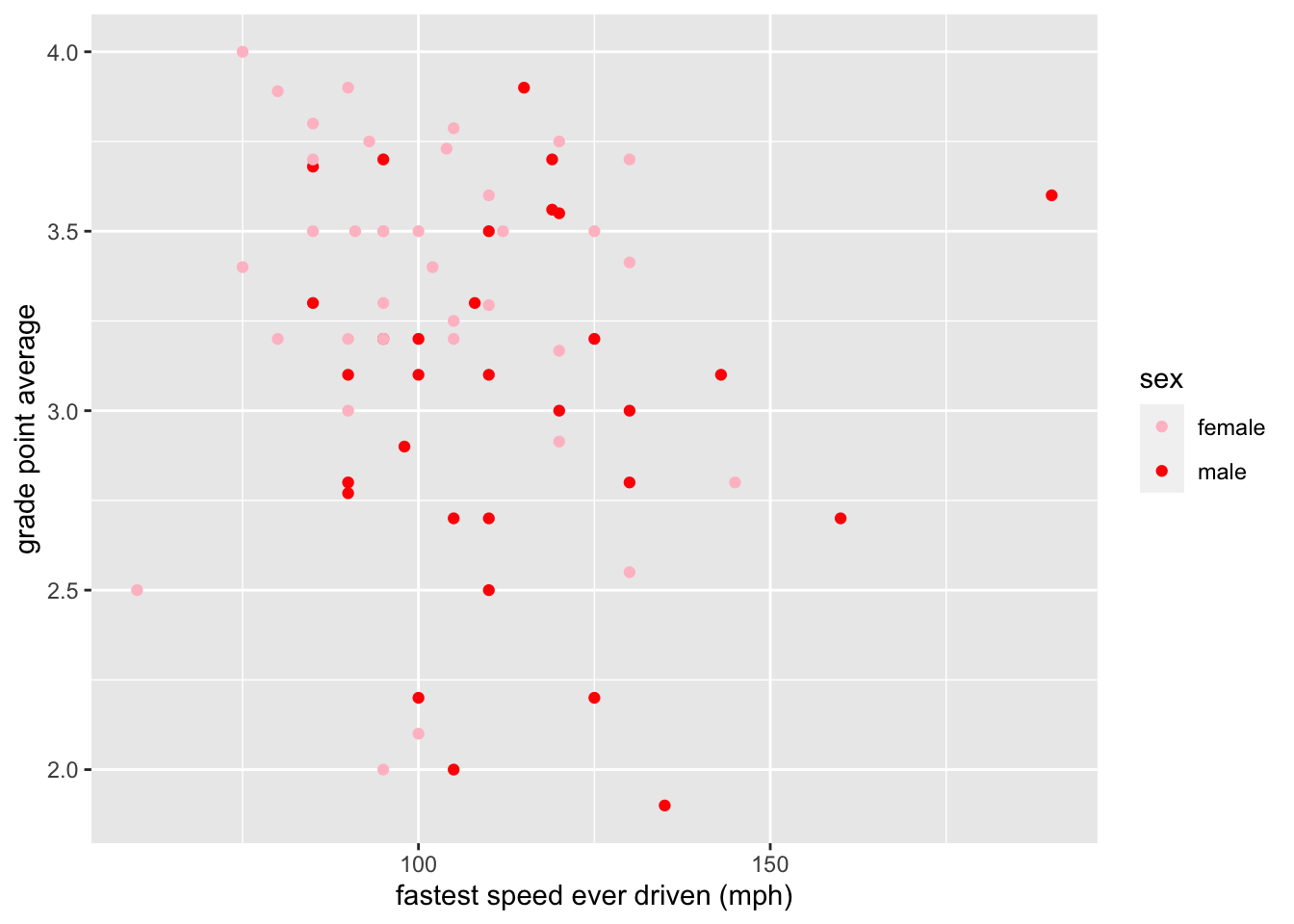

Figure 8.23: Color scale adjusted manually.

8.2.5 Layering: Adding Another Glyph Type

If you want to add another layer of glyphs, simply add on another call to a geom-function. In order to produce Figure 8.24, for example, we use the code below:

ggplot(m111survey, aes(x = seat, y = fastest)) + 
  geom_violin(fill = "burlywood") +
  geom_jitter(width = 0.2) +
  labs(x = "Seating preference",
       y = "Fastest speed ever driven (mph)",
             title = "There aren't so many back-sitters.")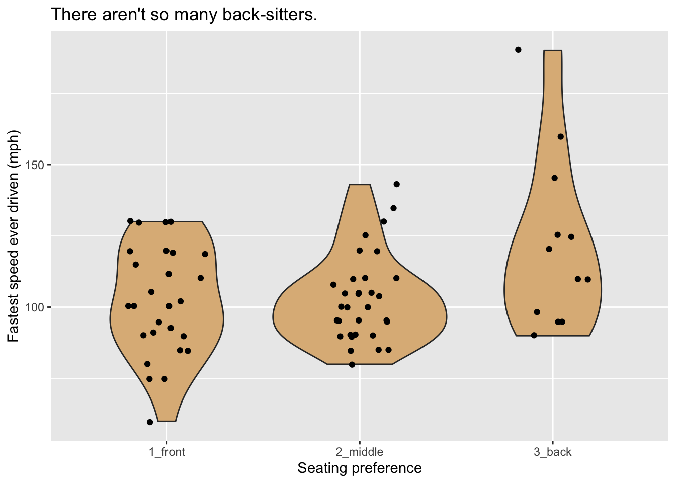

Figure 8.24: Violin plot of the fastest speed ever driven.

Note that the width parameter in the call to geom_jitter() determines how much the points are allowed to jitter horizontally.

8.2.5.1 Jitter-It-Yourself (JIY)

“Rug” glyphs are excellent, in especially in conjunction with density curves, but they have a downside. Consider, for example Figure 8.25 produced by the code below. When you examine the plot you will see that there aren’t as many rug-ticks as there are students in the m111survey data. Many students reported driving at the same speed, so their rug-ticks plotted over each other.

ggplot(m111survey, aes(x = fastest)) + 
  geom_density(fill = "burlywood") +
  geom_rug() +
  labs(x = "Fastest speed ever driven (mph)",
             title = "For most students the fastest speed is around 100 mph")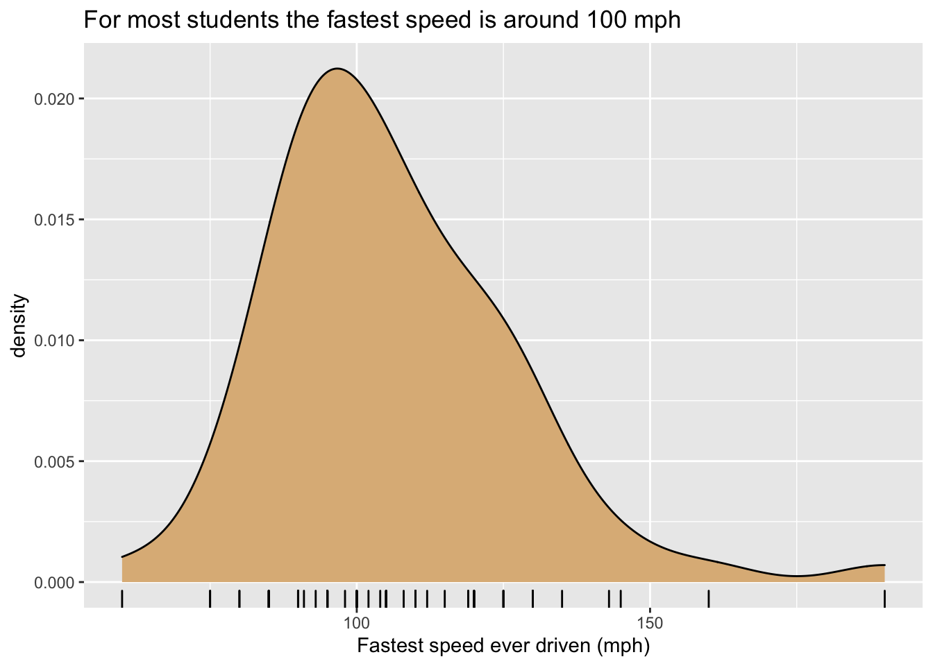

Figure 8.25: Density plot of the fastest speed ever driven. Some rug glyphs overplot each other.

It would be nice to solve the problem by jittering the rug-ticks, but unfortunately rug-ticks added to density plots don’t jitter nicely on their own. One reasonable workaround is to create one’s own randomly-jittered speeds and map the x-location of the rug-ticks to the new variable that holds the jittered values. The code below shows implements this idea, and results in Figure 8.26.

n <- nrow(m111survey)
m111survey$jitteredSpeeds <- m111survey$fastest + runif(n, -1, 1)
ggplot(m111survey, aes(x = fastest)) + 
  geom_density(fill = "burlywood") +
  geom_rug(aes(x = jitteredSpeeds)) +
  labs(x = "Fastest speed ever driven (mph)",
             title = "For most students the fastest speed is around 100 mph")

Figure 8.26: Density plot of the fastest speed ever driven. Rug glyphs are jittered.

8.2.6 Facets

As you will recall, a graph has facets when it is sub-divided into plots with one plot for each of the values of a categorical variable. ggplot2 has two functions to manage facet-ing:

facet_grid()
facet_wrap()

8.2.6.1 `facet_grid()`

The data frame railtrail from the bcscr package has information on usage of a converted railroad trail every day from April 5 to November 15, 2005. Study the Help file:

library(bcscr)

help(railtrail)

Every row in the data frame represents a particular day between April 5 and November 15.

Our goal is to study how the number of people on the trail on any given day relates to both the season and the time of week. This is a study of three variables together:

volume (number of people on the trail);
dayType (whether the day was a weekday or weekend);
season (whether the season was spring, summer or fall).

One possibility for a graph is to make a separate density plot of volume for each of the six possible combinations of values of the season and dayType variables. With facet_grid() we can arrange the plots in a grid so that the value of season is constant along rows and the value of dayType is constant along columns. This is accomplished by the following code, and the result appears as Figure 8.27.

ggplot(railtrail, aes(x = volume)) +
  geom_density(fill = "burlywood") +
  facet_grid(season ~ dayType)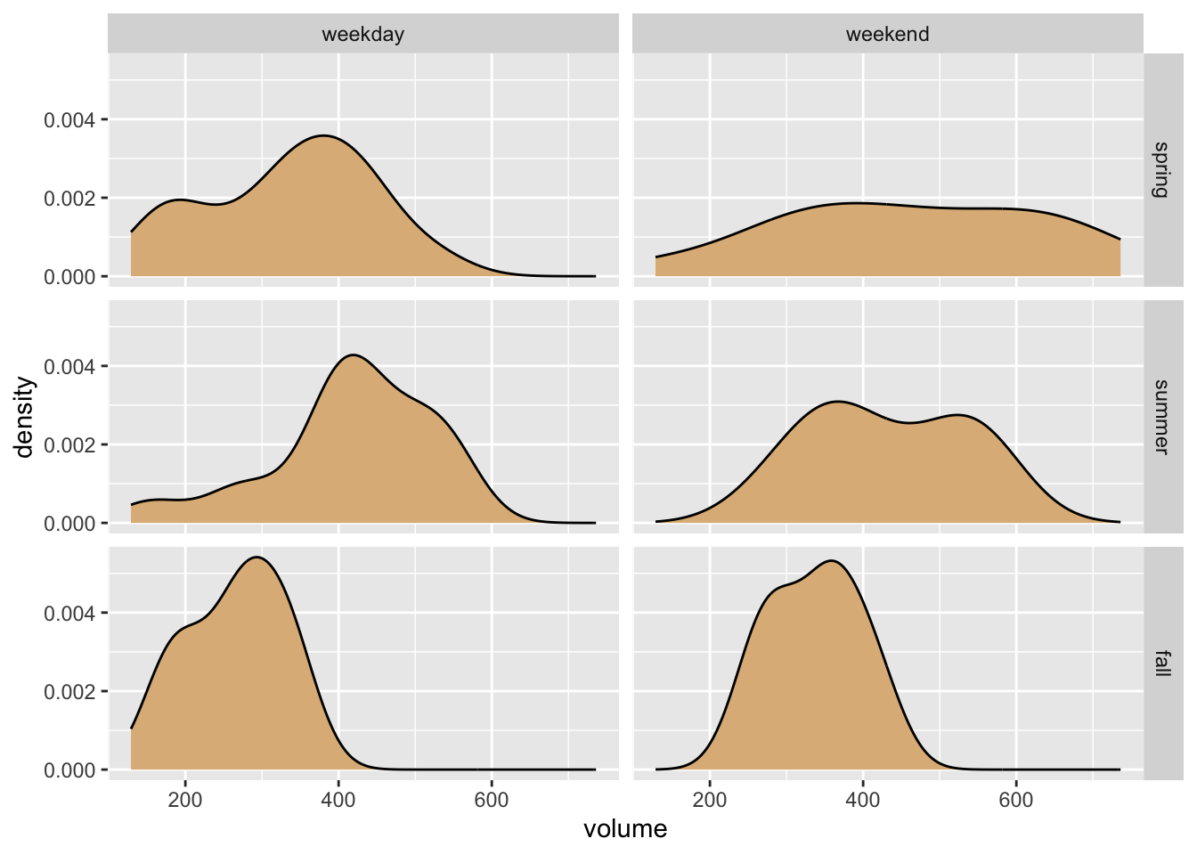

Figure 8.27: Volume of daily trail usage, by seaon and time of week.

Of course our aim is to see how volume varies with season and time of week, but the horizontal orientation of the volume variable in the above graph makes comparison difficult for most human viewers. Perhaps facet-ing in two dimensions was a bit too much, in this situation. In the code below, we produce a one-row, three-column layout in which each facet corresponds to one of the three seasons.²³ Within each facet, the days are broken down by time of week and volumes are compared with box plots. The result is seen in Figure 8.28. In the effort to incorporate the factor variables season and dayType into the graph, this second approach appears to strike a good balance between facet-ing and aesthetic mapping.

ggplot(railtrail, aes(x = dayType, y = volume)) +
  geom_boxplot(fill = "burlywood") +
  facet_grid( . ~ season) +
  labs(x = "Time of Week") +
  theme(legend.position = "top", legend.direction = "horizontal")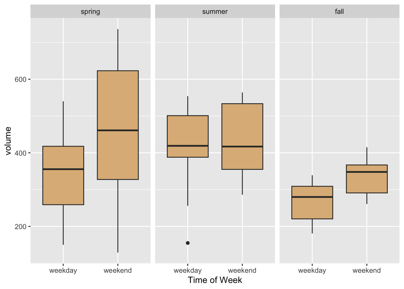

Figure 8.28: Striking a good balance between facet-ing and aesthetic mapping.

8.2.6.2 `facet_wrap()`

Frequently it happens that one desires to facet by a single categorical variable, and the number of levels of a factor variable is too large for the entire graph to be displayed well along a single row or a single column. In that event, use facet_wrap().

As an example, we will use the data table CPS85 from the mosaicData package:

library(mosaicData)

help("CPS85")

Each row is a worker, and the columns give information about their hourly wage, sector of employment, age, and so on.

Suppose, for example, that we want to compare the ages of workers in the eight different sectors of employment. Eight is a rather large number of plots, so we facet in “wrap-style” by means of the code below. The resulting plot appears as Figure 8.29.

ggplot(CPS85, aes(x = age)) +
  geom_density(fill = "burlywood") +
  facet_wrap(~ sector, nrow = 3)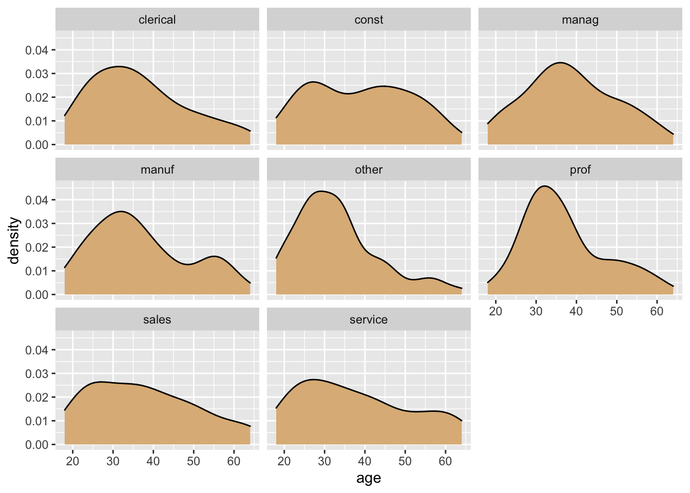

Figure 8.29: Age by sector.

Once again, though, it may be wise to consider an approach that involves aesthetic mapping. When the number of levels is large, violin plots or box plots may better approaches for representing a numerical variable such as age, as in the code below. The resulting graph is shown in Figure 8.30.

ggplot(CPS85, aes(x = sector, y = age)) +
  geom_boxplot(fill = "burlywood")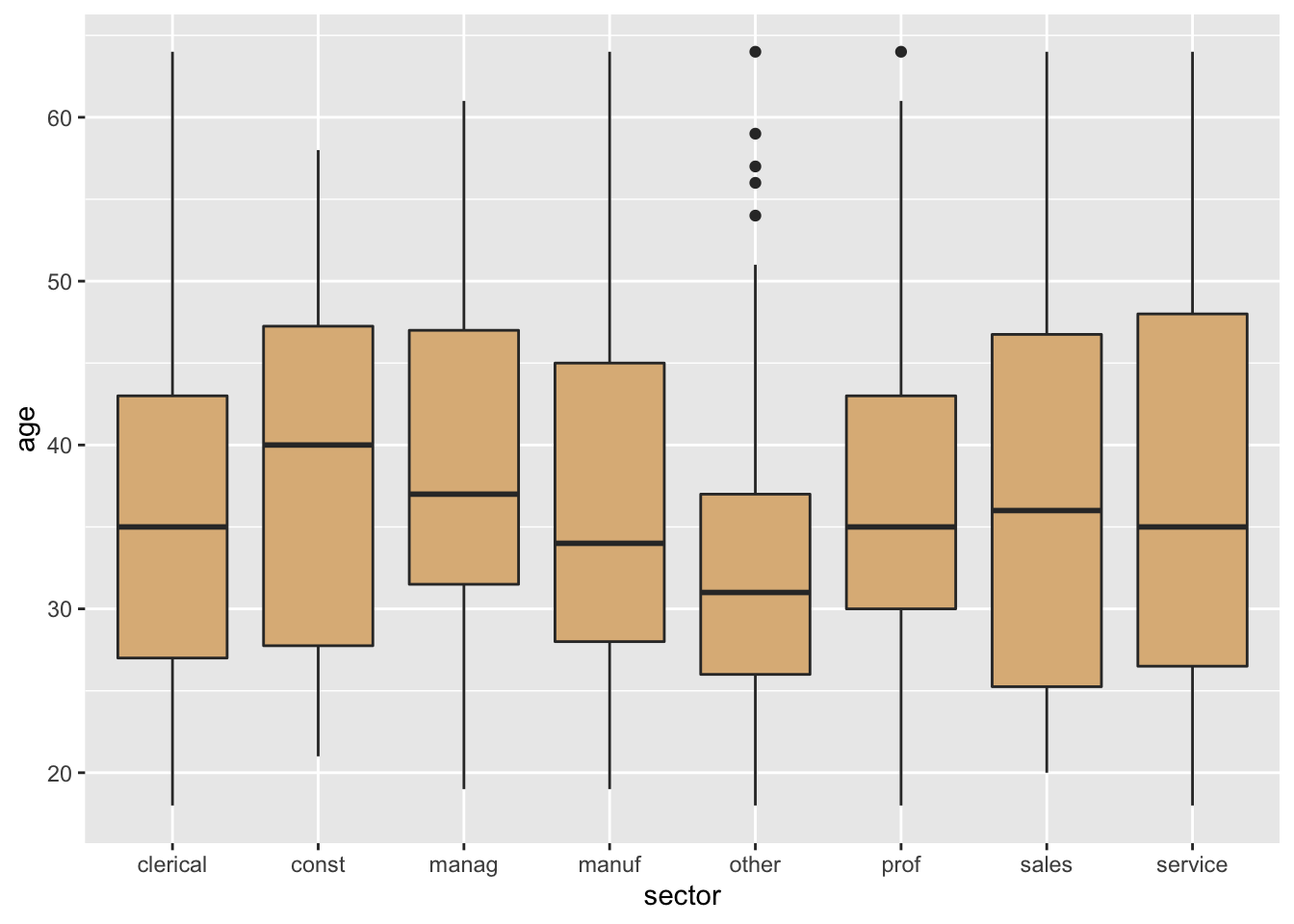

Figure 8.30: Aesthetic mapping is probably superior to facetting in this case.

In the exercises of this Chapter we will meet a case in which “wrap-style” facet-ing is quite useful.

8.2.7 Practice Exercises

With mosaicData::SwimRecords, make the following graph: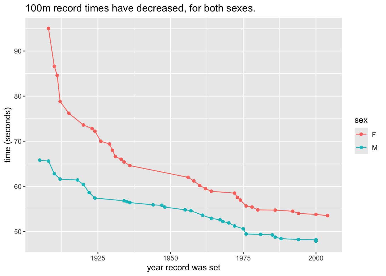
With bcscr::m111survey, make the graph below. (Hint: to get the squares, set the property shape to 22.)
With mosaicData::KidsFeet, make the following graph: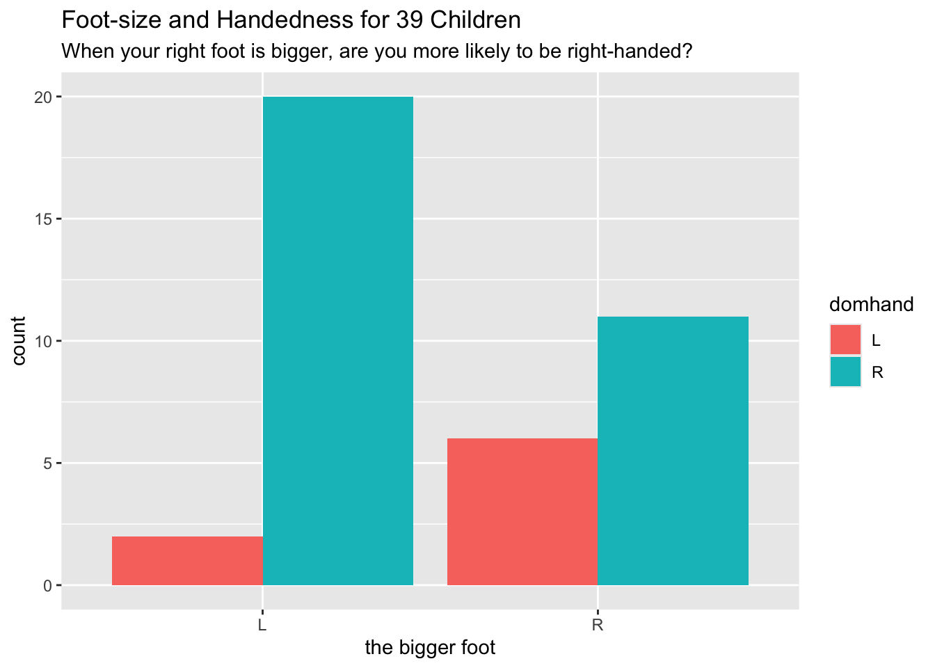
With mosaicData::TenMileRace, make the following graph: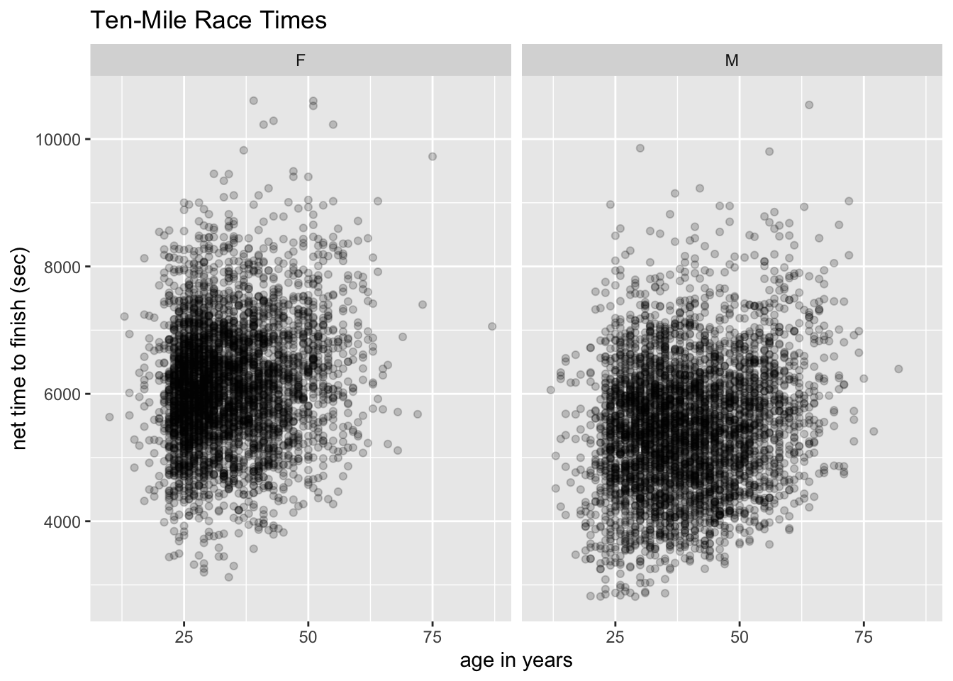

Hint: Make the call geom_point(alpha = 0.2). The alpha parameter has a default-value of 1. The lower you set it, the more “transparent” the points are. Low values for alpha are helpful to deal with the effects of “over-plotting” when many points are crowded together.
With mosaicData::Gestation make the following graph. The fill for the boxes is set to "burlywood". The x-location is mapped to factor(smoke), rather than to smoke.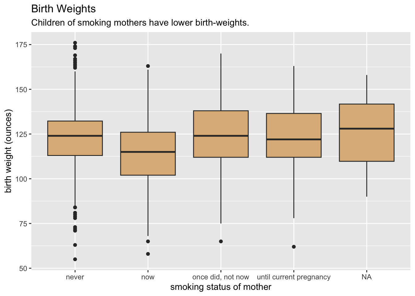
With mosaicData::Gestation make facet-ted histograms similar to the following, comparing the birth weights of babies born to mother who never smoked (“never”) vs. mothers who smoked during pregnancy (“now”). The fill for the rectangles is set to “skyblue”, and the color for the borders of the rectangles is set to “black”. The rectangles of a histogram are often called “bins”; the width of the rectangles is the “bin width”. If you do not set the binwidth property of the rectangles, ggplot2 will suggest in a message to the Console that you do so. Play with binwidth, adjusting it to a value that seems best for the data.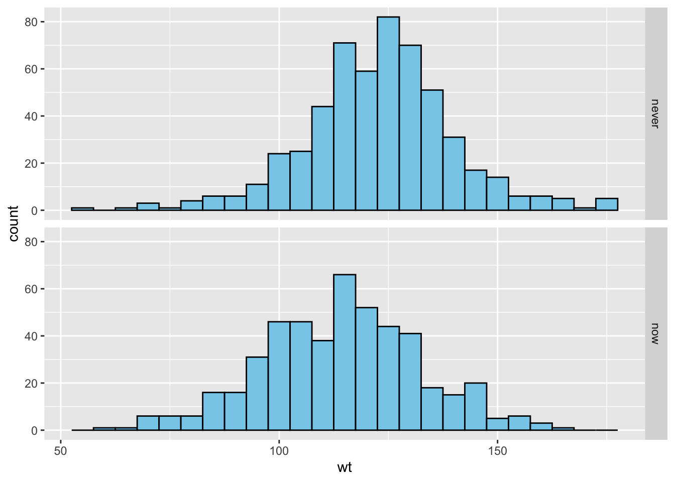
With mosaicData::Galton, make the following graph: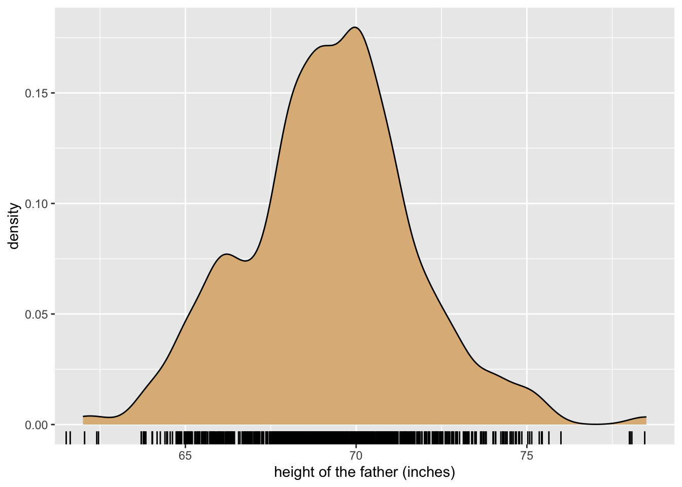

Hint: The fill of the density plot is set to "burlywood". The rug is made of randomly jittered father-heights.

8.2.8 Solutions to Practice Exercises

The call was:

ggplot(mosaicData::SwimRecords, aes(x = year, y = time)) +
  geom_point(aes(color = sex)) +
  geom_line(aes(color = sex)) +
  labs(x = "year record was set",
       y = "time (seconds)",
       title = "100m record times have decreased, for both sexes.")

The call was:

ggplot(bcscr::m111survey, aes(x = height, y = ideal_ht)) +
  geom_point(aes(color = weight_feel), shape = 22) +
  labs(
    x = "height (inches)",
    y = "ideal height (inches)",
    title = "The taller you are, the taller you want to be!",
    subtitle = "(Note: aesthetically mapping color to feeling about weight was silly!)"
  )

The call was:

ggplot(mosaicData::KidsFeet, aes(x = biggerfoot)) +
  geom_bar(aes(fill = domhand), position = "dodge") +
  labs(x = "the bigger foot",
       title = "Foot-size and Handedness for 39 Children",
       subtitle = paste0("When your right foot is bigger, ",
                         "are you more likely to be right-handed?"))

The call was:

ggplot(mosaicData::TenMileRace, aes(x = age, y = time)) +
  geom_point(alpha = 0.2) +
  facet_wrap(~ sex) +
  labs(x = "age in years", y = "net time to finish (sec)",
       title = "Ten-Mile Race Times")

The call was:

ggplot(mosaicData::Gestation, aes(x = factor(smoke), y = wt)) +
  geom_boxplot(fill = "burlywood") +
  labs(x = "smoking status of mother",
       y = "birth weight (ounces)",
       title = "Birth Weights",
       subtitle = "Children of smoking mothers have lower birth-weights.")

I settled on a bin width of 5 ounces:

df <- subset(
  mosaicData::Gestation,
  smoke %in% c("never", "now")
)

ggplot(df, aes(x = wt)) +
  geom_histogram(color = "black", fill = "skyblue", binwidth = 5) +
  labs("birth weight (ounces)") +
  facet_grid(smoke ~ .)

First, make the jittered points. It’s a good idea to load the data set directly, if you haven’t already attached mosaicData:

data("Galton", package = "mosaicData")

Now make the points:

jitteredFather <- Galton$father + runif(nrow(Galton), -0.5, 0.5)
Galton$jitteredFather <- jitteredFather

Finally, the graph:

ggplot(mosaicData::Galton, aes(x = father)) +
  geom_density(fill = "burlywood") +
  geom_rug(x = jitteredFather) +
  labs(x = "height of the father (inches)")

8.3 A Case Study: US Births

In Section 1.6, we made a plot of the number of births in the United States for each day of that year (see Figure 8.31). We noticed that there appear to be two clouds of points. What accounts for this phenomenon? By now we have the R-programming chops to take on this question.

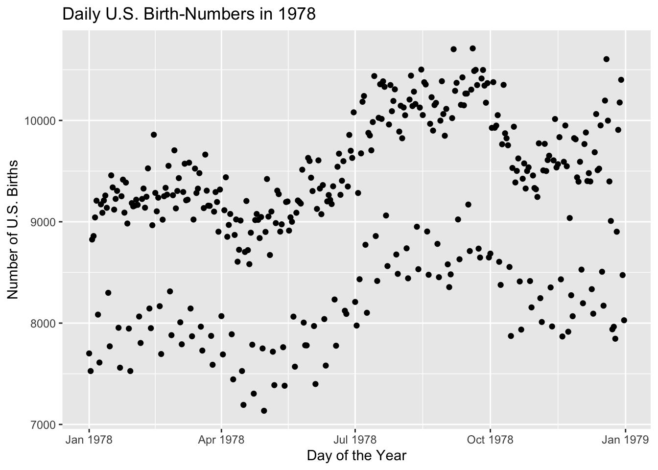
Figure 8.31: Some of the days have significantly fewer births. What’s going on?

To begin with, look at all of the variables available in the data frame Births78:

str(Births78)

## 'data.frame':    365 obs. of  8 variables:
##  $ date        : Date, format: "1978-01-01" ...
##  $ births      : int  7701 7527 8825 8859 9043 9208 8084 7611 9172 9089 ...
##  $ wday        : Ord.factor w/ 7 levels "Sun"<"Mon"<"Tue"<..: 1 2 3 4 5 6 7 1 2 3 ...
##  $ year        : num  1978 1978 1978 1978 1978 ...
##  $ month       : num  1 1 1 1 1 1 1 1 1 1 ...
##  $ day_of_year : int  1 2 3 4 5 6 7 8 9 10 ...
##  $ day_of_month: int  1 2 3 4 5 6 7 8 9 10 ...
##  $ day_of_week : num  1 2 3 4 5 6 7 1 2 3 ...

We see that the variable wday gives the name of the day of the week, for each of the days in the year. On a hunch, we make violin plots of the births for each of the days of the week. The code appears below, and the resulting plot is shown in Figure 8.32

ggplot(Births78, aes(x = wday, y = births)) + geom_violin(fill = "burlywood") +
  geom_jitter()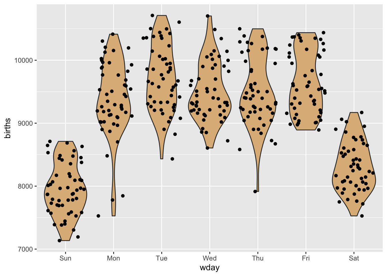

Figure 8.32: Violin plot of births, by day of the week.

Aha! There are considerably fewer births on the weekend-days—Saturday and Sunday. Perhaps the entire lower cloud of points is composed of weekends. Let’s check this by re-coding the days according to whether or not they are during the week or at the weekend:

weekend <- with(Births78, ifelse(wday %in% c("Sat","Sun"),
                                 "weekend", "weekday"))
Births78$weekend <- weekend

Note that we have added the new variable to the data frame, so that it will be easy in ggplot2 to use that variable for grouping, as in the code below. The results appear in Figure 8.33.

ggplot(Births78, aes(x = date, y = births)) + geom_point(aes(color = weekend)) +
  labs(x = "Day of the Year", y = "Number of U.S. Births",
       title = "Daily U.S. Birth-Numbers in 1978")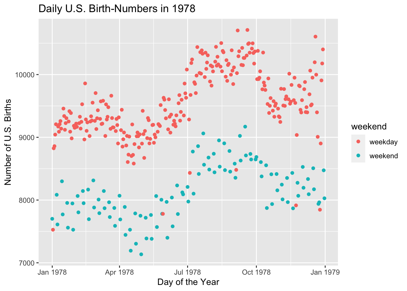

Figure 8.33: The days with fewer births are almost always weekend-days.

Well, a few of the points in the lower cloud are weekdays. Is there anything special about them? To find out, we subset the data frame to examine only those points:

df <- subset(Births78, weekend != "weekend" & births <= 8500)
df

##           date births wday year month day_of_year day_of_month
## 2   1978-01-02   7527  Mon 1978     1           2            2
## 149 1978-05-29   7780  Mon 1978     5         149           29
## 185 1978-07-04   8433  Tue 1978     7         185            4
## 247 1978-09-04   8481  Mon 1978     9         247            4
## 327 1978-11-23   7915  Thu 1978    11         327           23
## 359 1978-12-25   7846  Mon 1978    12         359           25
##     day_of_week weekend
## 2             2 weekday
## 149           2 weekday
## 185           3 weekday
## 247           2 weekday
## 327           5 weekday
## 359           2 weekday

If you consult a calendar for the year 1978, you will find that every one of the above days was a major holiday. Apparently doctors prefer not to deliver babies on weekend and holidays. Scheduled births—induced births or births by non-emergency Cesarean section—are not usually set for weekends or holidays. Perhaps this accounts for the two clouds we saw in the original scatter plot.

8.3.1 Practice Exercises

With mosaicData::KidsFeet, make the following graph. (Hint: Use plyr::mapvalues().)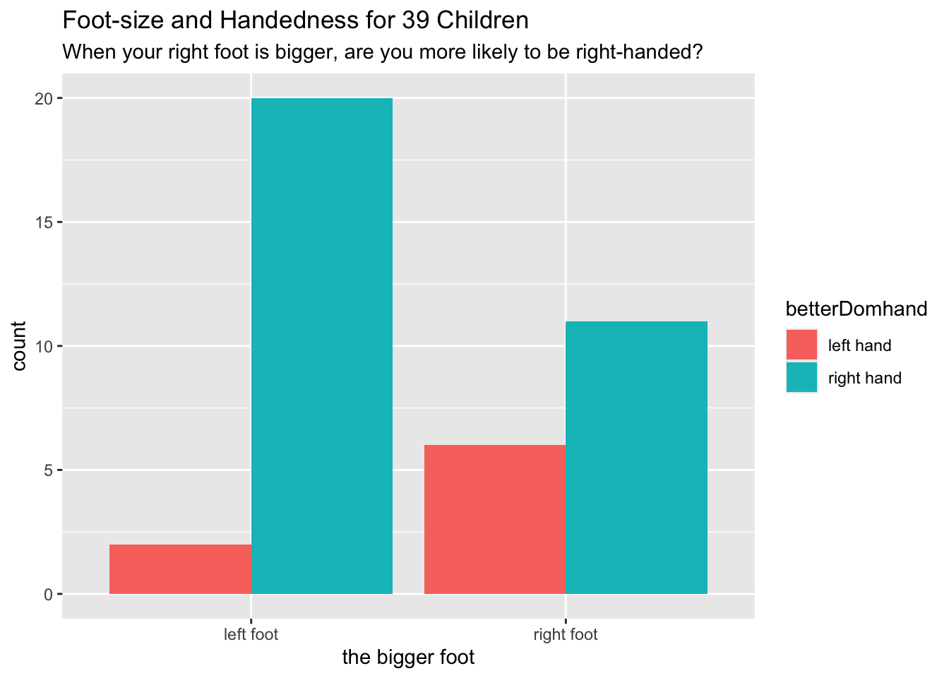
With mosaicData::TenMileRace, make the following graph. (Hint: Use cut() to make age groups. The fill for the boxes is the ever-popular "burlywood".)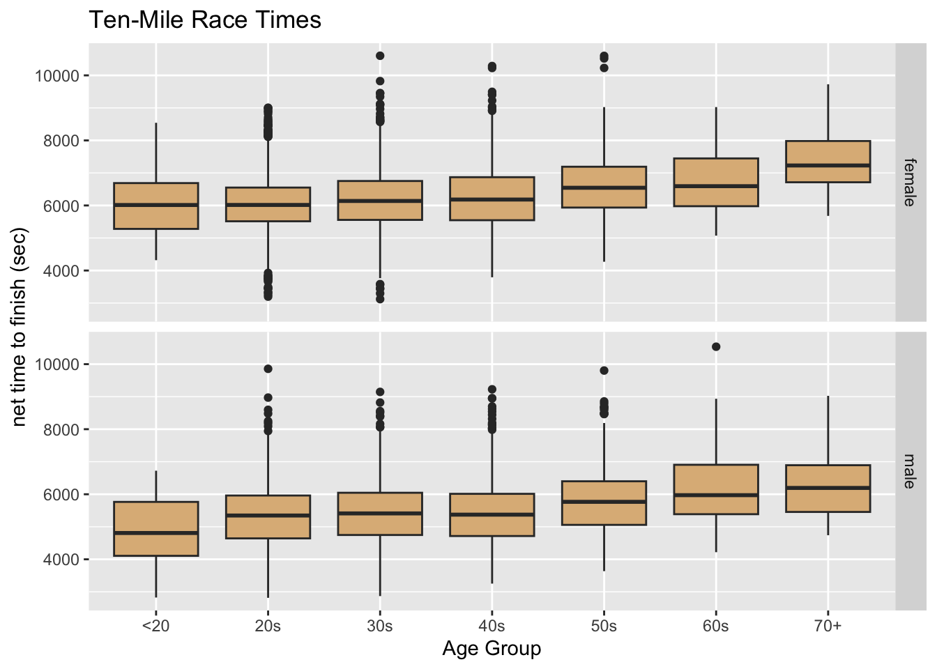
With mosaicData::Gestation, make the following graph. (Hint: Use !is.na() to select the rows of Gestation where smoke is not NA. Then use plyr::mapvalues() on smoke.)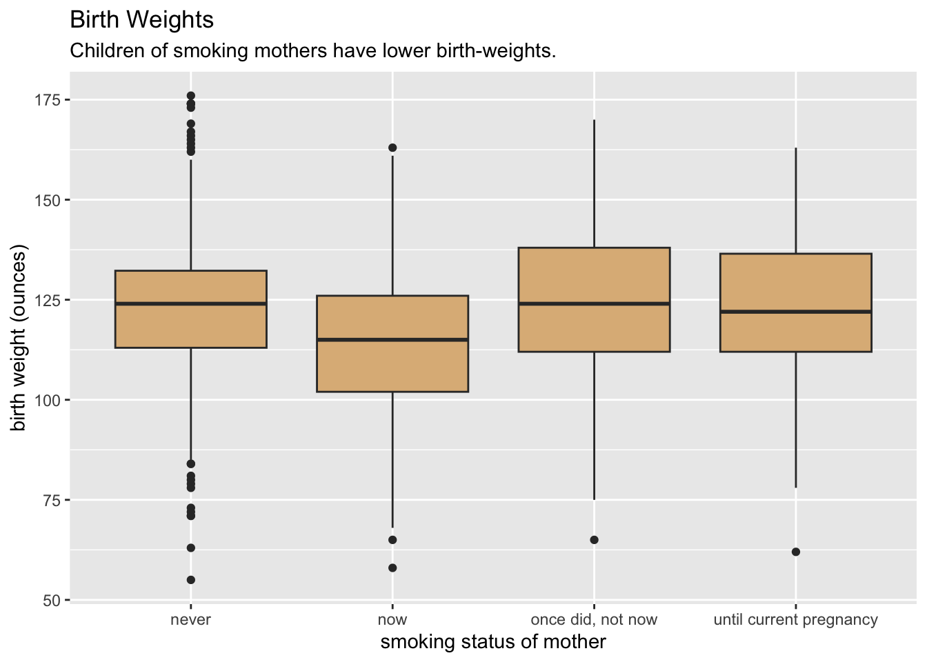

8.3.2 Solutions to Practice Exercises

Here’s the code:

data("KidsFeet", package = "mosaicData")
tempBiggerfoot <- KidsFeet$biggerfoot
biggerfoot2 <- plyr::mapvalues(tempBiggerfoot, c("L", "R"),
                     to = c("left foot", "right foot"))
KidsFeet$betterBiggerfoot <- biggerfoot2
tempDomhand <- KidsFeet$domhand
domhand2 <- plyr::mapvalues(tempDomhand, from = c("L", "R"),
                     to = c("left hand", "right hand"))
KidsFeet$betterDomhand <- domhand2
ggplot(KidsFeet, aes(x = betterBiggerfoot)) +
  geom_bar(aes(fill = betterDomhand), position = "dodge") +
  labs(x = "the bigger foot",
       title = "Foot-size and Handedness for 39 Children",
       subtitle = paste0("When your right foot is bigger, ",
                         "are you more likely to be right-handed?"))

Here’s the code:

data("TenMileRace", package = "mosaicData")
tempSex <- TenMileRace$sex
sex2 <- plyr::mapvalues(tempSex, from = c("F", "M"),
                       to = c("female", "male"))
TenMileRace$betterSex <- sex2
ageGroup <- cut(TenMileRace$age,
                breaks = c(-Inf, 20, 30, 40, 50, 60, 70, Inf),
                labels = c("<20", "20s", "30s", "40s", 
                           "50s", "60s", "70+"))
TenMileRace$ageGroup <- ageGroup
ggplot(TenMileRace, aes(x = ageGroup, y = time)) +
  geom_boxplot(fill = "burlywood") +
  facet_grid(betterSex ~ .) +
  labs(x = "Age Group", y = "net time to finish (sec)",
       title = "Ten-Mile Race Times")

Here’s the code:

data("Gestation", package = "mosaicData")
Gestation <- subset(Gestation, !is.na(smoke))
tempSmoke <- Gestation$smoke
smoke2 <- plyr::mapvalues(tempSmoke, from = 0:3,
                         to = c("never", "smokes now",
                                "until curr. preg.",
                                "once smoked"))
Gestation$betterSmoke <- smoke2
ggplot(Gestation, aes(x = factor(betterSmoke), y = wt)) +
  geom_boxplot(fill = "burlywood") +
  labs(x = "smoking status of mother",
       y = "birth weight (ounces)",
       title = "Birth Weights",
       subtitle = "Children of smoking mothers have lower birth-weights.")

8.4 Learn More

From time to time we will return to ggplot2 and deepen our study of this remarkable graphing system. If you are impatient to learn more right way, you can explore the package’s documentation site. The site teaches the system by way of numerous examples that you can copy and modify.

8.5 More in Depth

8.5.1 Factor Variables in Plotting

It is worthwhile to reconsider factor variables (see 7.4.3) and to consider their role in the appearance of plots. We’ll do this by way of an example.

Consider the data frame firesetting in the tigerData package:

data("firesetting", package = "tigerData")
?tigerData::firesetting

As we see from the Help file, fire-setting offers information about a large sample of high-school students. Some of them are known to be arsonists, while of course most are not. The purpose for gathering the data was to determine what characteristics of a child might be risk factors in whether he/she would develop into a fire-setter. Among the variables of interest are:

race, the ethnicity of the student, a factor with three levels: “white”, “black”, and “other”;
school.attitude, a scaled score on a personality inventory in which high scores indicate a poor attitude toward school;
fires, a factor variable with levels “0” (does not set fires) and “1” (sets fires).

We might study the relationship between these variables with some box-plots via the code below. The results appear as Figure 8.34.

ggplot(firesetting, aes(x = race, y = school.attitude)) +
  geom_boxplot(fill = "burlywood", 
               outlier.alpha = 0) + 
  geom_jitter(width = 0.20, size = 0.1) +
  facet_wrap(~ fires, nrow = 2) +
  labs(x = "Ethnicity",
       y = "School-Attitude Score")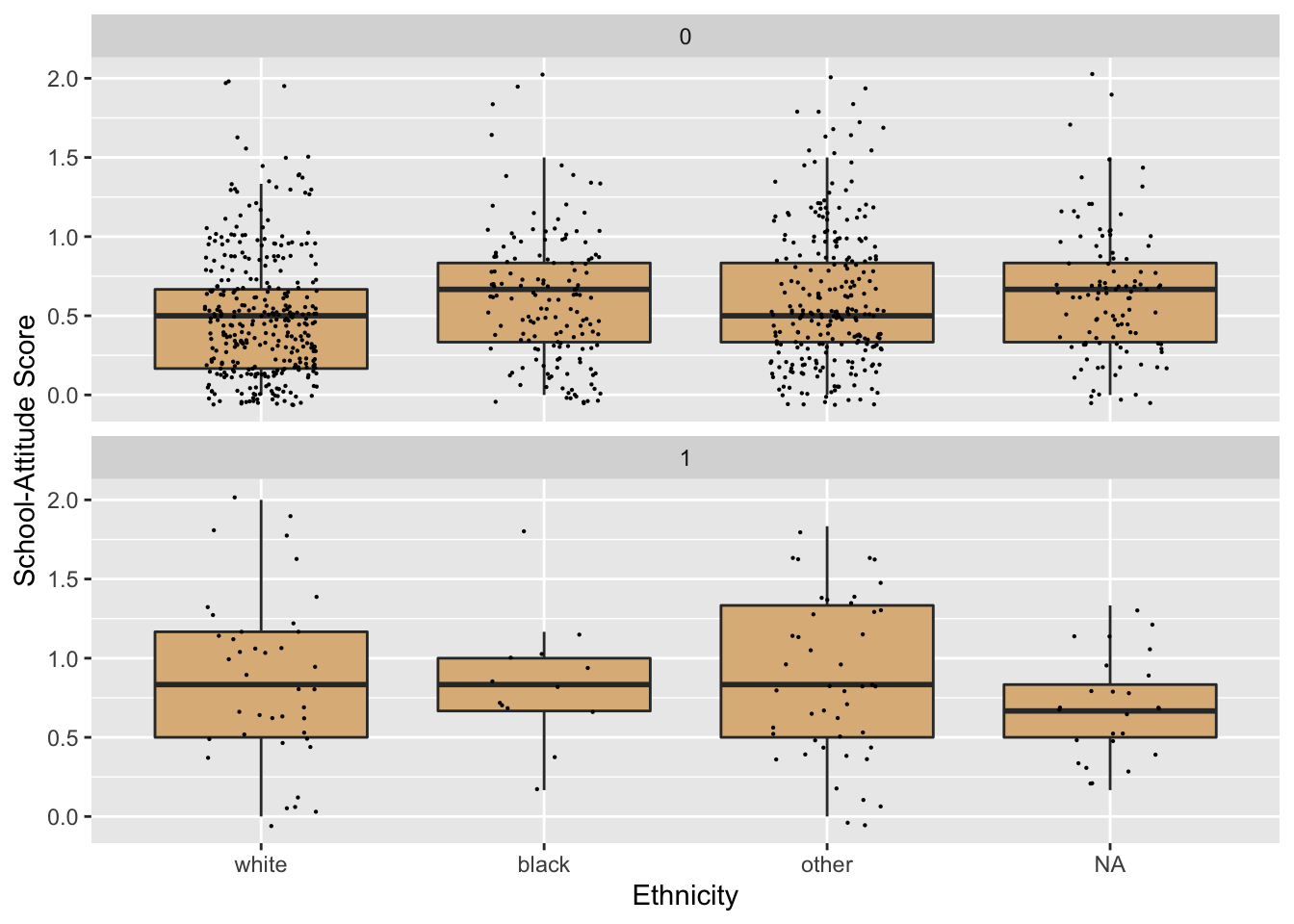

Figure 8.34: Boxplots with jittered individual values. School attitudes are generally worse among fire-setters.

We could improve the appearance of the plot with respect to two of the variables involved:

fires: We should display values that are more meaningful to a human viewer than 0 and 1.
race: Let’s change the names of the values somewhat, keeping their current order along the x-axis.

For fires, we simply need to map the current values onto others that we prefer. Currently the levels are:

levels(firesetting$fires)

## NULL

We can re-map as follows:

betterFires <- plyr::mapvalues(firesetting$fires, from = c("0", "1"),
                         to = c("no fires", "sets fires"))
firesetting$betterFires <- betterFires

For race, we’d like to substitute

“White” for “white”;
“AfrAm” for “black”
“Other” for “other”
“Unknown” instead of NA

We’d like the order along the horizontal axis to remain as it is.

We might begin by replacing the NA-values with “Unknown”, as follows:

tempRace <- firesetting$race
tempRace[is.na(tempRace)] <- "Unknown"

We get an error! That’s because race is a factor with only three “possible values”, as given by its levels:

levels(tempRace)

## [1] "white" "black" "other"

“Unknown” is not considered a “possible value” for tempRace, any attempt to set that value in any elements of tempRace will be resisted.

We can overcome this resistance by coercing tempRace into a mere character-vector:

tempRace <- as.character(tempRace)

Now tempRace doesn’t come with a limit on its “possible values”. We try again:

tempRace[is.na(tempRace)] <- "Unknown"

This apparently worked. Let’s check:

unique(tempRace)

## [1] "white"   "other"   "Unknown" "black"

So far, so good. Now let’s re-map the other three values:

tempRace2 <- plyr::mapvalues(tempRace,
                        from = c("white", "black", "other"),
                        to = c("White", "AfrAm", "Other"))

Let’s check that it worked:

unique(tempRace2)

## [1] "White"   "Other"   "Unknown" "AfrAm"

Great. Now let’s add tempRace2 as a new variable into firsetting. In that data frame, it will be called betterRace. Here’s the code to do this:

firesetting$betterRace <- tempRace2

Let’s try the graph again. We will need to modify the code a bit, so that we’re using the new and improved variable betterRace, as well as the new variable betterFires. Figure 8.35 is the result.

ggplot(firesetting, aes(x = betterRace, y = school.attitude)) +
  geom_boxplot(fill = "burlywood", 
               outlier.alpha = 0) + 
  geom_jitter(width = 0.20, size = 0.1) +
  facet_wrap(~ betterFires, nrow = 2) +
  labs(x = "Ethnicity",
       y = "School-Attitude Score")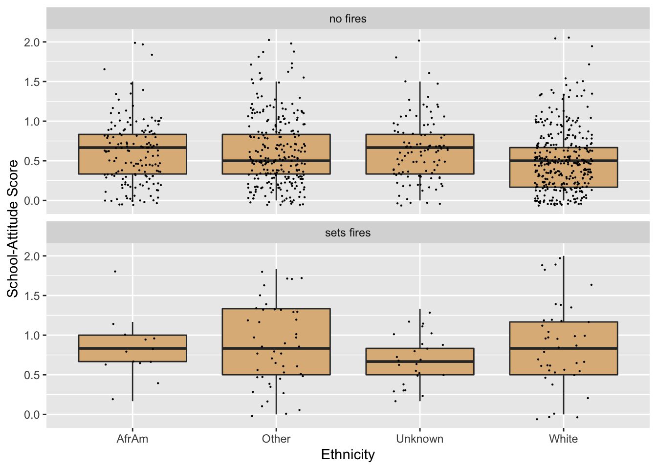

Figure 8.35: We have re-mapped the fires and race variables.

This looks better, but now the order along the x-axis isn’t as we desired. Recall that race is now a character vector only. Since it doesn’t have levels that specify a particular order, ggplot2 uses alphabetical order as the default ordering along the x-axis.

Accordingly we should convert betterRace to a factor variable, and be careful to set the levels in the order that we want:

tempRace <- firesetting$betterRace
betterRace2 <- factor(tempRace,
               levels = c("White", "AfrAm", "Other", "Unknown"))
firesetting$evenBetterRace <- betterRace2

Now try again. Note that in the code below we switch to evenBetterRace. See Figure 8.36 for the result.

ggplot(firesetting, aes(x = evenBetterRace, y = school.attitude)) +
  geom_boxplot(fill = "burlywood", 
               outlier.alpha = 0) + 
  geom_jitter(width = 0.20, size = 0.1) +
  facet_wrap(~ betterFires, nrow = 2) +
  labs(x = "Ethnicity",
       y = "School-Attitude Score")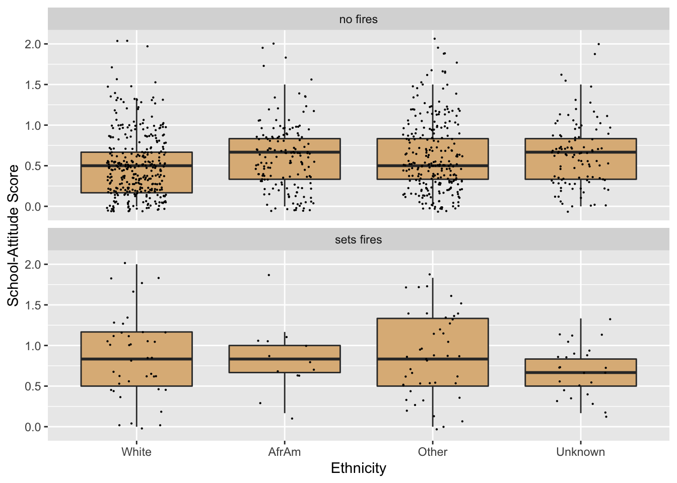

Figure 8.36: Now the order of the race-values is correct!

This works!

8.5.2 Example: Dental Floss

If you are like me, you don’t like to run out of an item that you commonly use, so you always try to have a spare source for the item on hand. Take dental floss, for example. It’s difficult to know when the little box is almost out of floss. Hence I try to keep two boxes on hand in my bathroom drawer: the one I’m using, and a spare. The problem is that I can never tell which one is “the one I’m using” and which one is the spare. In fact on any given day I’m equally likely to pull a length of floss out of either one of the boxes.²⁴

Let’s make the following assumptions:

A box of floss starts out with 150 feet of floss.
I start with two fresh boxes.
Every time I floss, each box has a 50% chance of being the box I pull from.
When I pull out floss, the length I choose to pull is a random number between 1 and 2 feet. If the box has less than than the amount I choose to pull, then I will just pull out whatever if left.

There are several interesting questions we could ask concerning this situation. In this example, let’s focus on finding the expected value of $X$, the amount of floss left in the other box when I discover that one of the boxes is exhausted.

I would also like to get some idea of the distribution of $X$—the chance for it to assume each of its possible values. Unlike many random variables that we have studied previously $X$ is what we call a continuous random variable: it can assume any of the values in a range of real numbers. After all, the amount left in the “other” box could be anything from 0 to 150 feet: it could be 3.5633 feet or 5.21887 feet, or any real number at all, so long as it’s between 0 and 150. Although any real number value—3.5633 feet, for instance—is possible, it seems that the chance of $X$ being exactly 3.5633 is vanishingly small, and the same goes for any of the possible real numbers value for $X$. Hence it seems that the distribution of $X$ cannot be described well with a table of the values that we actually get in a simulation: indeed, we are highly unlikely to get any value more than once in the course of our simulation.

One way to visualize the distribution of a continuous random variable is to make a density plot of a large, representative sample of its values. Let’s practice making a density plot for a random variable that R provides for us: a so-called normal random variable. Try this code:

x <- rnorm(100, mean = 70, sd = 3)

We have just asked R to produce 100 numbers chosen randomly from a normal distribution. The mean parameter sets what the values should be “on average”, and the sd parameter indicates how much they should typically differ from that average value. The bigger the sd, the bigger the difference between the mean and value actually obtained is liable to be.

Let’s get a look at the first ten values in the vector x:

x[1:10]

##  [1] 71.13092 70.90465 66.70593 66.60878 61.61040 72.16172 72.81736
##  [8] 69.31187 75.27739 70.35210

Sure enough, the numbers are typically around the mean of 70, give or take 3 units or so.

We can use the ggplot2 package to produce a density curve from all 100 values in the vector x. (The resulting plot appears as Figure 8.37.)

p <- ggplot(mapping = aes(x = x)) + geom_density() + geom_rug() +
  labs(x = "x-value")
p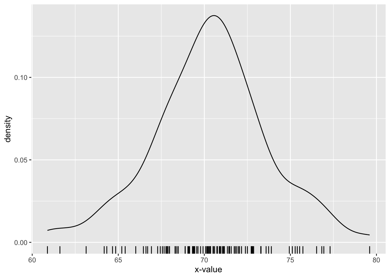

Figure 8.37: Density plot of 100 random values from a normal distribution with mean 70 and standard deviation 3.

The density plot gives us a visual sense of the distribution of the normal random variable: it seems rather likely to come out between 67 and 73 (most of the area under the curve occurs there) and rather unlikely to be greater than 76, and so on.

In a similar way, we can get a sense of the distribution of the the $X$, the length of floss left in the remaining box, if we simulate its values many times.

Since we have worked through the encapsulation-and-generalization development process a number of times by now, we will simply show a final-form implementation of a simulation function called floss_sim(). This function takes the following parameters:

reps: number of simulations (default 1000);
len: the initial length of floss in any unused box (default-value is 150);
min_pull: the minimum length I could choose to pull (default value is 1);
max_pull: the maximum length of floss that I could choose to pull (default value is 2);
graph: if TRUE, show show a density plot of the simulated values of $X$ (default value FALSE;)
seed: the usual option to set a random seed.

The function returns an estimated of the expected value of $X$.

floss_sim <- function(reps = 1000, len = 150, 
                     min_pull = 1, max_pull = 2,  
                     graph = FALSE, seed = NULL) {
  if ( !is.null(seed) ) {
    set.seed(seed)
  }
  # helper-function to remove floss from a box:
  new_length <- function(current_length) {
    desired_amount <- runif(1, min = min_pull, max = max_pull)
    max(0, current_length - desired_amount)
  }
  
  # vector to hold the simulated leftover-box lengths:
  leftover <- numeric(reps)
  # now the simulations.  Each time we loop through, we
  # start with two fresh boxes and use them until
  # one runs out.
  for (i in 1:reps ) {
    # set up two fresh boxes:
    box <- c(len, len)
    # now floss away!
    repeat {
      # determine which box is picked
      picked <- sample(c(1, 2), size = 1)
      box[picked] <- new_length(box[picked])
      if (any(box <= 0)) {
        remaining <- max(box)
        leftover[i] <- remaining
        break
      }
    }  # end repeat-loop
  }    # end for loop
  if (graph) {
    plot_title <- paste(
      "Dental-Floss Simulation with ", 
      reps, " Repetitions", sep =""
    )
    sim_plot <- ggplot(mapping = aes(leftover)) + 
      geom_density(fill = "burlywood") +
      labs(
        x = "Amount in remaining box (ft)",
        title = plot_title
      )
     print(sim_plot)
  }
  # return estimate:
  mean(leftover)
}

Let’s give it a try with one thousand repetitions.

floss_sim(graph = TRUE, seed = 3535)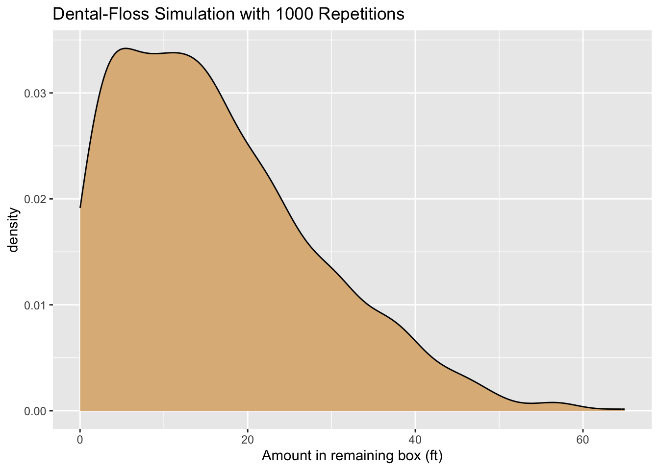

Figure 8.38: Density plot of the results of a dental-floss simulation.

## [1] 16.3279

A density plot of the results appears as Figure 8.38. The expected value of the amount left in the remaining box is about 16.3 feet, but you can see from the plot that there is some variability: it’s not all that unlikely to have 40 or more feet left!

8.5.3 Example: The Drunken Turtle

Let us return to the scenario of the Drunken Turtle that was introduced in Section 5.4.5. At each step the turtle would turn by a random angle—any angle between 0 and 360 degrees with equal likelihood—and then move forward by a fixed number of units. We wondered whether the turtle would simply wander away from its starting point or perhaps eventually loop back close to its starting point.

In this section we will construct a simulation that sheds light on our question. We will imagine that the turtle starts at the origin on the $xy$-plane and takes a large but fixed number of steps—one thousand steps, say—each of a fixed length of one unit, but each of which is preceded by a drunken turn through a random angle. We will concern ourselves with the random variable $X$, defined as follows:

$X$ = the number of times in the turtle returns to within $1/2$ of a unit of the origin, during its first 1000 steps.

(Apparently we consider a “close return” to be anything within half a unit of the origin.)

In particular, we would like to know the distribution of $X$: what is the chance that the turtle does not make a close return during the first thousand steps? What’s the chance of making only one close return? Two close returns? And so on … . We would also like to estimate the expected value of $X$: the average number of close returns in the first 1000 steps.

We will next consider how to code a simulation. Obviously we will need a way to record the turtle’s position at each step. In order to accomplish this we will have to apply the unit-circle trigonometry you learned in high school.

Instead of measuring angles in degrees, we will work in radians: by default R does trigonometry that way. Recall that 360 degrees is $2 \pi$ radians; hence the way to determine the angle of a turn by the drunken turtle is with the following call to runif():

runif(1, min = 0, max = 2*pi)

## [1] 5.052785

If we want a thousand drunken turn-angles, then we can get them all in a vector, as follows:

runif(1000, min = 0, max = 2*pi)

So much for the turning angles. But in order to decide at each step whether the turtle has made a close return, we have to know the coordinates of the turtle after each step. This is where unit-circle trigonometry comes in handy. Recall that if a right triangle has a hypotenuse of length 1 (the length of a turtle step) and if one of the angles of the triangle is $\alpha$, then the side adjacent to $\alpha$ is $\cos(\alpha)$ and the side opposite is $\sin(\alpha)$. The situation is illustrated in Figure 8.39.

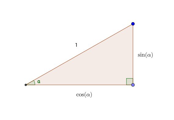
Figure 8.39: Sides of a right triangle with hypotenuse 1, in terms of the angle shown.

From this principle it follows that if the turtle turns a random angle of $a_1$ radians for its first step, then after it takes the one-unit step it will be at the point $(\cos(a_1), \sin(a_2))$.

For the second step, the turtle begins by turning another random angle, say $a_2$ radians. It then takes another one-unit step. This second step forms the hypotenuse of a second right triangle (see Figure 8.40). The horizontal and vertical sides of this right triangle must be $\cos(a_2)$ and $\sin(a_2)$ respectively. When the turtle complete the second step, it has added these values to its previous $x$ and $y$ coordinates, so that it is now at the point:

\[(\cos(a_1) + \cos(a_2), \sin(a_1) +\sin(a_2)).\] We now see the idea: in order to record the position of the turtle at the end of each step, we simply need to:

take the cosine of all the turning-angles;
take the sine of all the turning-angles;
sum the cosines to get the $x$-coordinate;
sum the sines to get the $y$-coordinate.

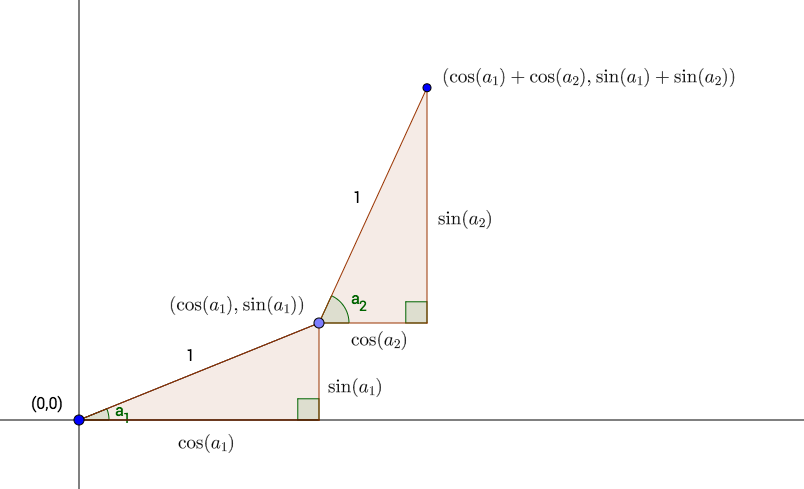
Figure 8.40: The first two steps by the Drunken Turtle. Turtle turns by $a_1$ radians for Step One, then by $a_2$ radians for Step Two.

Let’s put this idea into practice, for just the first ten steps. First, get the turning angles, the sines and the cosines:

angle <- runif(10, 0 , 2*pi)
xSteps <- cos(angle)
ySteps <- sin(angle)

Next, we need to add the xSteps together. If we do a sum, we would get the $x$-coordinate after the tenth step:

sum(xSteps)

## [1] -1.370258

(Apparently some of the cosines were negative, meaning that some of the turning angles were between 90 and 270 degrees.)

We need the $x$-coordinates after all of the previous steps, as well. This can be accomplished with R’s cumsum() function. You may think of cumsum as short for “cumulative sum”. Given a vector vec of numbers, cumsum(vec) returns a vector of the same length, where for every index i, cumsum(vec)[i] is sum(vec[1:i]). This is made clear in the following example:

vec <- c(3, 2, -1, 4, -2)
cumsum(vec)

## [1] 3 5 4 8 6

Look at the table below.

`vec`	cumulative sum	`cumsum(vec)`
3	3	3
2	$3+2$	5
-1	$3+2+-1$	4
4	$3+2+-1+4$	8
-2	$3+2+-1+4+-2$	6

See how it works?

Returning to xSteps, we see that we can get the $x$-coordinates of the first ten steps like this:

x <- cumsum(xSteps)
x

##  [1] -0.6034165 -1.3905805 -2.1259607 -3.1154380 -2.4593130
##  [6] -1.5476110 -0.8591924 -1.6420445 -0.6421761 -1.3702583

Similarly we can get the first ten $y$-coordinates:

y <- cumsum(ySteps)

Using the distance formula, we can compute the distance of each point from the origin as follows:

dist <- sqrt(x^2 + y^2)

The following logical vector will then record, at each each step, whether or not the turtle has made a close return:

closeReturn <- (dist < 0.5)

The results are shown in Table 8.2.

Table 8.2: Record of the turtle’s first ten steps. It has not yet made a close return.
angle	xSteps	ySteps	x	y	dist	closeReturn
4.0646104	-0.6034165	-0.7974262	-0.6034165	-0.7974262	1.000000	FALSE
2.4769935	-0.7871641	0.6167437	-1.3905805	-0.1806826	1.402270	FALSE
3.8861615	-0.7353801	-0.6776548	-2.1259607	-0.8583374	2.292695	FALSE
2.9963954	-0.9894774	0.1446876	-3.1154380	-0.7136497	3.196131	FALSE
0.8551238	0.6561251	0.7546522	-2.4593130	0.0410024	2.459655	FALSE
0.4233886	0.9117020	0.4108522	-1.5476110	0.4518546	1.612226	FALSE
0.8114898	0.6884186	0.7253136	-0.8591924	1.1771682	1.457373	FALSE
2.4700328	-0.7828521	0.6222079	-1.6420445	1.7993761	2.435993	FALSE
0.0162276	0.9998683	0.0162269	-0.6421761	1.8156030	1.925826	FALSE
3.8968689	-0.7280822	-0.6854899	-1.3702583	1.1301131	1.776165	FALSE

It remains only to package our code into a simulation function. We will allow the user to specify the fixed initial number of steps (it does not have to be 1000), and also to determine what distance counts as a “close return.”

drunken_sim <- function(steps = 1000, reps = 10000, 
                        close = 0.5, seed = NULL, 
                        table = FALSE) {
  if ( !is.null(seed) ) {
    set.seed(seed)
  }
  # set up returns vector to store the number of 
  # close returns in each repetition:
  returns <- numeric(reps)
  
  for (i in 1:reps) {
    # get all the turning angles:
    angle <- runif(steps, 0 , 2*pi)
    # all the changes in x-coordinate of turtle:
    xSteps <- cos(angle)
    # all changes in the y-coordinate:
    ySteps <- sin(angle)
    # x and y coordinates at each step of the journey:
    x <- cumsum(xSteps)
    y <- cumsum(ySteps)
    ## all the distances
    dist <- sqrt(x^2 + y^2)
    ## whether or not you are close to (0,0),
    ## at each step:
    is_close <- (dist < close)
    ## count the number of times turtle was close:
    close_returns <- sum(is_close)
    returns[i] <- close_returns
  }
  
  if ( table ) {
    cat("Here is a table of the number of close returns:\n\n")
    tab <- prop.table(table(returns))
    print(tab)
    cat("\n")
  }
  mean(returns)
}

Let’s try it out, where the journey is goes on for one thousand steps and a return is considered to be “close” when the turtle is less than 0.5 units from its starting point.

drunken_sim(steps = 1000, reps = 10000, 
           close = 0.5, seed = 3535, table = TRUE)

## Here is a table of the number of close returns:
## 
## returns
##      0      1      2      3      4      5      6      7      8 
## 0.3881 0.2290 0.1517 0.0908 0.0572 0.0335 0.0227 0.0107 0.0064 
##      9     10     11     12     13     14     15     16     17 
## 0.0048 0.0018 0.0012 0.0008 0.0007 0.0003 0.0001 0.0001 0.0001

## [1] 1.5655

Notice that 38.81% of the time the turtle did not make a close return at all during the first thousand steps. On the other hand it is possible, though not at all likely, for the turtle to make quite a few close returns.²⁵

It is interesting to look specifically at the distances from the origin. The following function draws a graph of the distance from the origin for the specified number of turtle steps:

drunken_sim_2 <- function(steps = 1000, seed = NULL) {
  if ( !is.null(seed) ) {
    set.seed(seed)
  }
  angle <- runif(steps, 0 , 2*pi)
  xSteps <- cos(angle)
  ySteps <- sin(angle)
  x <- cumsum(xSteps)
  y <- cumsum(ySteps)
  dist <- sqrt(x^2 + y^2)
  plot_title <- paste(
    "First ", steps, 
    " Steps of the Drunken Turtle",
    sep = ""
  )
  dist_plot <- ggplot(mapping = aes(x = 1:steps, y=dist)) + 
    geom_line() +
    labs(
      x = "Step", 
      y = "Distance From Origin",
      title = plot_title)
  print(dist_plot)
}

Let’s try it out! The results appear in Figure 8.41

drunken_sim_2(steps = 1000, seed = 2525)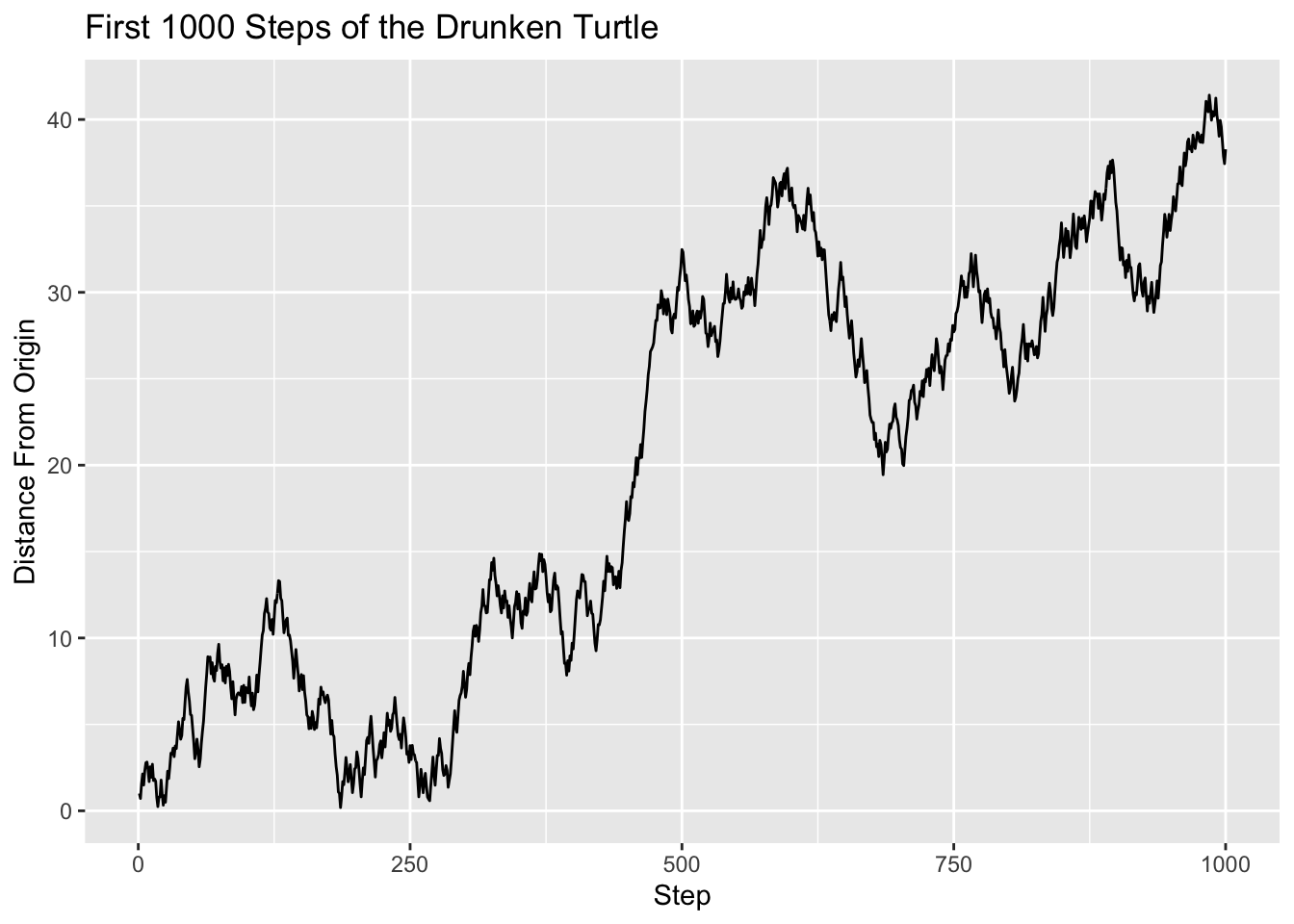

Figure 8.41: Line plot of the Turtle’s distance from the origin, as a function of how many steps the turtle has taken.

It appears that although the turtle might have returned close to the origin a couple of times, for the most part it seems to be wandering further and further away. In the mathematical field known as stochastic processes, it has been shown that if the turtle is allowed to go on forever then it will certainly make a close return infinitely many times—no matter how narrowly one defines “close”! Nonetheless, as our graph suggests, the close returns tend to be spaced further and further apart as time goes on.

8.5.4 Practice Exercises

In a previous Practice Exercise (see Section 6.8.5), you wrote a function called freeThrowSim() to estimate the probability that in 20 attempts you will make more shots than Lester does. Write a new version of the function that offers the option to view a histogram of the simulated differences (number you make minus number Lester makes).

8.5.5 Solutions to the Practice Exercises

Here you go:

freeThrowSim <- function(reps, seed, shots,
                         you = 0.70, lester = 0.60,
                         graph = FALSE) {
      youMake <- rbinom(reps, size = shots, prob = you)
      lesterMakes <- rbinom(reps, size = shots, prob = lester)
      youWin <- (youMake > lesterMakes)
      diffs <- youMake - lesterMakes
      df <- data.frame(diffs = diffs)
      if (graph) {
        diff_plot <- 
          ggplot(df, aes(x = diffs)) +
          geom_histogram(
            color = "black", fill = "skyblue", 
            binwidth = 1
          ) +
          labs(x = "difference (you minus Lester)")
        print(diff_plot)
      }
      mean(youWin)
    }

The Main Ideas of This Chapter

The main features of the Grammar of Graphics:
- Frame
- Glyphs
- Aesthetics
- Scales
- Guides
ggplot() makes the frame.
Add more elements to a plot with +.
Glyphs come from functions that start with geom. The following are especially common:
- geom_bar()
- geom_histogram()
- geom_density()
- geom_boxplot()
- geom_violin()
- geom_point()
When you represent your data with more than one type of glyph, you are *layering”. Common layering examples:
- geom_density() (or geom_histogram()) with geom_rug();
- geom_boxplot() (or geom_violin()) with geom_jitter().
Don’t forget to make good axis-labels with labs().
Facet-ing is done with facet_grid() or facet_wrap().
Often you must manipulate your data set—for example, select only certain rows from it, or add a new column to it—prior to making your graph.

Links to Class Slides

Quarto Presentations that I sometimes use in class:

Glossary

Frame: The aesthetics (usually x and y position) that help locate cases on a plot.
Glyph: The basic graphical unit that corresponds to a case in the data table.
Aesthetic: A perceptible property of a glyph that varies from case to case.
Scale: The relationship between the value of a variable and the graphical attribute to be displayed for that value.
Guide: An indication, for the human viewer, of the scale being used in an aesthetic mapping.

Exercises

Using the bcscr::m111survey data frame, write the ggplot2 code necessary to produce the graph in the figure below. (The points are all blue.)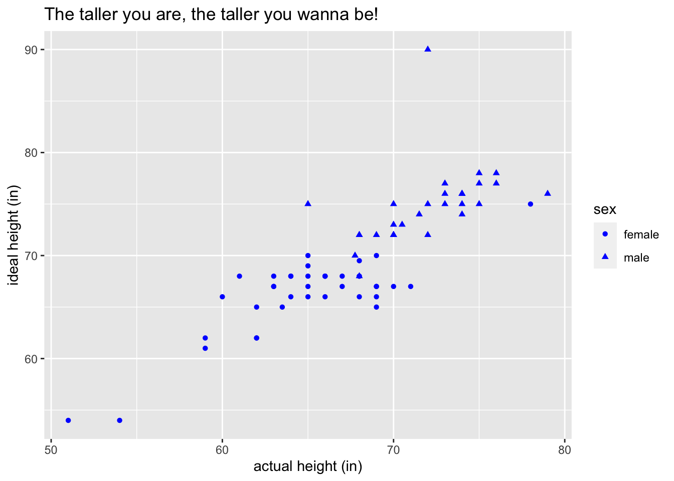

Hint: For the points, map the aesthetic property shape to the variable sex. On the other hand, color is a fixed property in this graph.
Using the mosaicData::Utilities data frame, write the ggplot2 code necessary to produce the graph in the figure below.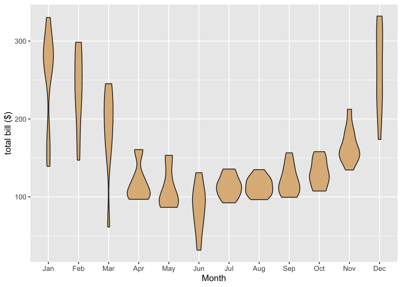

Hint: The month variable in Utilities is given numerically: 0 for January, 1 for February, and so on. You’ll need to use plyr::mapvalues() to map the numbers from 1 to 12 to the abbreviated month names. (See section 8.5.1 for a review of this.) The special R-vector month.abb will render the re-mapping task easy:
```
month.abb
```
```
##  [1] "Jan" "Feb" "Mar" "Apr" "May" "Jun" "Jul" "Aug" "Sep" "Oct"
## [11] "Nov" "Dec"
```
In fact, you can create a new variable with abbreviated monnths, using this code:
```
monthAbbr <- plyr::mapvalues(
  Utilities$month,
  from = 1:12,
  to = month.abb
)
```
You also need to make sure that the months come in the right order along the x-axis of the graph. To do this consider resetting the levels of your new monthAbbr variable. One way to accomplish this is to convert monthAbbr back to a factor with levels in the order you want, as done in Section 8.5.1, like this:
```
monthAbbr <- factor(monthAbbr, levels = month.abb)
```
Then you can put your new variable into the data frame, naming it anything you like:
```
Utilities$monthName <- monthAbbr
```
The next few exercises pertain to the data frame CPS85 from the package mosaicData. Learn about it with help(CPS85). We will use the ggplot2 graphing package to explore whether men were being paid more than women in 1985.

Make a density plot of the wages of the people in the study. As with all plots you make, it should have well-labelled axes (with units if possible). For a density plot you should label the horizontal axis, but you can let ggplot2 provide the label for the “density” axis. As always, provide a descriptive title. Also provide a “rug” of individual values along the horizontal axis.
Look at the plot you made in the previous exercise: you will notice that one person made a wage that was much higher than all the rest. In data analysis, when a value is much higher or lower than the rest of the values we call it an outlier.

Write the code needed to find the age, sex and sector of employment of the person who made this extraoridinarily high wage. Report the age, sex and sector of this person.

Create a new data frame called cpsSmall that is the same as CPS85 except that it excludes the row corresponding to the outlier-individual.
In order to explore the relationship between wage and sex in the CPS study, make violin plots for the wages of men and women. (In this exercise and in subsequent exercises, use the cpsSmall data frame so as to exclude the outlier.) Based on the plot, who tends to earn higher wages: men or women?
(*) Someone might argue that men don’t earn higher wages because of sex-discrimination in the workplace, but rather because of some other factor. For example, it could be that in 1985 women chose to work in low-wage sectors of the economy, whereas men tended to work in higher-wage sectors. Of course for this explanation to be viable, some sectors of the economy have to pay more on average than other sectors do. In order to verify whether this is the case, make a box plot of wage vs. sector of employment. Use the plot to name a couple of high-wage sectors and a couple of low-wage sectors.
(*) From the previous exercise you now know that some sectors of the economy pay more than other sectors. Hence in order to investigate properly whether there was wage-discrimination in the workforce based on sex, we would have to compare the wages of men and women who work in the same sector. To this end it would be nice to have eight separate box plots, one for each sector. Each plot would compare the wages of men and women in that sector. Use facet_wrap() to construct a graph that displays all eight plots at once.

Examine your graph.
- Are there any sectors in which it seems that women typically make more than men. If so, what sectors are they?
- On the other hand, are there any sectors where men typically make more than women? If so, what sectors are they?
- Based on your analysis, does it seem plausible that women made less than men simply because they chose lower-paying sectors of employment?

7 Data Frames

9 Lists

`vec`	cumulative sum	`cumsum(vec)`
3	3	3
2	\(3+2\)	5
-1	\(3+2+-1\)	4
4	\(3+2+-1+4\)	8
-2	\(3+2+-1+4+-2\)	6

8 Graphics

8.1 The Grammar of Graphics

8.1.1 Example: a Scatterplot

8.1.1.1 The Glyphs

8.1.1.2 The Aesthetics

8.1.1.3 The Frame

8.1.1.4 Scales

8.1.1.5 Guides

8.1.1.6 Summary

8.1.2 Example: Two Bar Graphs

8.1.3 Examples: Histograms, Density Plots and Box Plots

8.1.3.1 Histograms

8.1.3.2 Density Plots

8.1.3.3 Box Plots

8.1.4 Example: Choropleth Maps

8.1.5 Practice Exercises

8.1.6 Solutions to Practice Exercises

8.2 Implementation in ggplot2

8.2.1 Basic Setup: the Data Frame

8.2.2 More Setup: Establishing the Frame

8.2.3 Labels

8.2.4 Adding a Type of Glyph

8.2.4.1 Our First Geoms

8.2.4.2 Further Aesthetic Mappings

8.2.4.3 Aesthetic Mappings vs. Fixed Properties

8.2.4.4 Adjusting Scales

8.2.5 Layering: Adding Another Glyph Type

8.2.5.1 Jitter-It-Yourself (JIY)

8.2.6 Facets

8.2.6.1 facet_grid()

8.2.6.2 facet_wrap()

8.2.7 Practice Exercises

8.2.8 Solutions to Practice Exercises

8.3 A Case Study: US Births

8.3.1 Practice Exercises

8.3.2 Solutions to Practice Exercises

8.4 Learn More

8.5 More in Depth

8.5.1 Factor Variables in Plotting

8.5.2 Example: Dental Floss

8.5.3 Example: The Drunken Turtle

8.5.4 Practice Exercises

8.5.5 Solutions to the Practice Exercises

The Main Ideas of This Chapter

Links to Class Slides

Glossary

Exercises

8.2.6.1 `facet_grid()`

8.2.6.2 `facet_wrap()`