4.4 Application: The Collatz Conjecture

Take any positive integer greater than 1. Apply the following rule, which we will call the Collatz Rule:

• If the integer is even, divide it by 2;
• if the integer is odd, multiply it by 3 and add 1.

Now apply the rule to the resulting number, then apply the rule again to the number you get from that, and so on.

For example, start with 13. We proceed as follows:

• 13 is odd, so compute \(3 \times 13 + 1 = 40\).
• 40 is even, so compute \(40/2 = 20\).
• 20 is even, so compute \(20/2 = 10\).
• 10 is even, so compute \(10/2 = 5\).
• 5 is odd, so compute \(3 \times 5+ 1 = 16\)
• 16 is even, so compute \(16/2 = 8\).
• 8 is even, so compute \(8/2 = 4\).
• 4 is even, so compute \(4/2 = 2\).
• 2 is even, so compute \(2/2 = 1\).
• 1 is odd, so compute \(3 \times 1 + 1 = 4\).
• 4 is even, so compute \(4/2 = 2\).
• 2 is even, so compute \(2/2 = 1\).

If we keep going, then we will cycle forever:

\[4, 2, 1, 4, 2, 1, \ldots\] In mathematics the Collatz Conjecture is the conjecture that for any initial positive number, every Collatz Sequence (the sequence formed by repeated application of the Collatz Rule) eventually contains a 1, after which it must cycle forever. No matter how large a number we begin with, we have always found that it returns to 1, but mathematicians do not know if this will be so for any initial number.

A sequence of Collatz numbers can bounce around quite remarkably before descending to 1. Our goal in this section is to write a function called collatz() that will compute the Collatz sequence for any given initial number and draw a graph of the sequence as well.

First, let’s make a function just for the Collatz Rule itself:

collatzRule <- function(m) {
  if ( m %% 2 == 0) {
    return(m/2)
  } else {
    return(3*m + 1)
  }
}

(Recall that m %% 2 is the remainder of m after it is divided by 2. If this is 0, then m is even.)

Next let’s try to get a function going that will print out Collatz numbers:

collatz <- function(n) {
  # n is the initial number
  while ( n > 1 ) {
    cat(n, " ", sep = "")
    # get the next number and call it n:
    n <- collatzRule(n)
  }
}

Let’s try it out:

collatz(13)

## 13 40 20 10 5 16 8 4 2

So far, so good, but if we are going to graph the numbers, then we should store them in a vector. The problem is that we don’t know how long the vector needs to be.

One possible solution is to add to the vector as we go, like this:

collatz <- function(n) {
  numbers <- numeric()
  while ( n > 1 ) {
    # stick n onto the end of numbers:
    numbers <- c(numbers, n)
    n <- collatzRule(n)
  }
  print(numbers)
}

Try it out:

collatz(13)

## [1] 13 40 20 10  5 16  8  4  2

This looks good. There are two problems, though, if the Collatz sequence happens to go on for a very long time.

• Computation Time: the user doesn’t know when the sequence will end—if ever!—so she won’t know whether a delay in production of the output is due to a long sequence or a problem with the program itself. as the sequence gets longer, the computation-time is made even longer by the way the following line of code works:

  numbers <- c(numbers, n)

  R cannot actually “stick” a new element onto the end of a vector. What it actually does is to move to a new place in memory and create an entirely new vector consisting of all the elements of numbers followed by the number n. R then assigns the name numbers to this value, freeing up the old place in memory where the previous numbers vector lived, but when a vector is very long copying can take a long time.

• Memory Problems Once the numbers vector gets long enough it will use all of the memory in the computer that is available to R. R will crash.

In order to get around this problem, we should impose a limit on the number of Collatz numbers that we will compute. We’ll set the limit at 10,000. The user can change the limit, but should exercise caution in doing so. Also, we’ll initialize our numbers vector to have a length set to this limit. We can then assign values to elements of an already existing vector: this is much faster than copying entire vectors from scratch.

collatz <- function(n, limit = 10000) {
  # collatz numbers will go in this vector
  numbers <- numeric(limit)
  # keep count of how many numbers we have made:
  counter <- 0
  while ( n > 1 & counter < limit) {
    # need to make a new number
    counter <- counter + 1
    # put the current number into the vector
    numbers[counter] <- n
    # make next Collatz number
    n <- collatzRule(n)
  }
  # find how many Collatz numbers we made:
  howMany <- min(counter, limit)
  # print them out:
  print(numbers[1:howMany])
}

Again let’s try it:

collatz(257)

##   [1]  257  772  386  193  580  290  145  436  218  109  328  164   82   41  124   62
##  [17]   31   94   47  142   71  214  107  322  161  484  242  121  364  182   91  274
##  [33]  137  412  206  103  310  155  466  233  700  350  175  526  263  790  395 1186
##  [49]  593 1780  890  445 1336  668  334  167  502  251  754  377 1132  566  283  850
##  [65]  425 1276  638  319  958  479 1438  719 2158 1079 3238 1619 4858 2429 7288 3644
##  [81] 1822  911 2734 1367 4102 2051 6154 3077 9232 4616 2308 1154  577 1732  866  433
##  [97] 1300  650  325  976  488  244  122   61  184   92   46   23   70   35  106   53
## [113]  160   80   40   20   10    5   16    8    4    2

Things are working pretty well, but since the sequence of numbers might get pretty long, perhaps we should only print out the length of the sequence, and leave it to the reader to say whether the sequence itself should be shown.

collatz <- function(n, limit = 10000) {
  numbers <- numeric(limit)
  counter <- 0
  while ( n > 1 & counter < limit) {
    counter <- counter + 1
    numbers[counter] <- n
    n <- collatzRule(n)
  }
  howMany <- min(counter, limit)
  cat("The Collatz sequence has ", howMany, " elements.\n", sep = "")
  show <- readline("Do you want to see it (y/n)?  ")
  if ( show == "y" ) {
    print(numbers[1:howMany])
  }
}

Next let’s think about the plot. We’ll use the plotting system in the ggplot2 package (Wickham et al. 2020).

library(ggplot2)

Later on we will make a serious study of plotting with ggplot2, but for now let’s just get the basic idea of plotting a set of points. First, let’s get a small set of points to plot:

xvals <- c(1, 2, 3, 4, 5)
yvals <- c(3, 7, 2, 4, 3)

xvals contains the x-coordinates of our points, and yvals contains the corresponding y-coordinates.

We set up a plot as follows:

ggplot(mapping = aes(x = xvals, y = yvals))

The ggplot() function sets up a basic two-dimensional grid. The mapping parameter explains how data will be “mapped” to particular positions on the plot. In this case it has been set to:

aes(x = xvals, y = yvals)

aes is short for “aesthetics,” which has to do with how somethings looks. The expression means that xvals will be located on the x-axis and yvals will be located on the y-axis of the plot.

Now let’s see what we get if we actually run the call to the ggplot() function (see Figure 4.2):

ggplot(mapping = aes(x = xvals, y = yvals))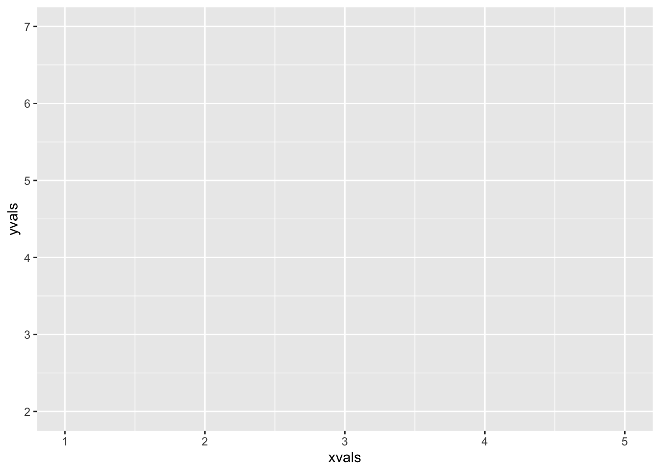

Figure 4.2: A ggplot2 plot without geoms.

The plot is blank! Why is this? Well, although ggplot() has been told what values are to be represented on the plot and where they might go, it has not yet been told how they should be shaped: it has not been told their geometry, you might say. We can add a geometry to the plot to get a picture (see Figure 4.3:

ggplot(mapping = aes(x = xvals, y = yvals)) +
  geom_point()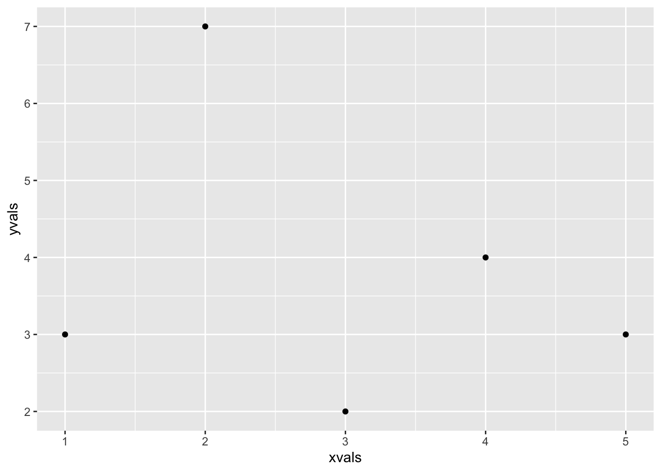

Figure 4.3: A ggplot2 plot with the point geom.

The geometry determines a lot about the look of the plot. In order to have the points connected by lines we could add geom_line() (see Figure 4.4:

ggplot(mapping = aes(x = xvals, y = yvals)) +
  geom_point() +
  geom_line()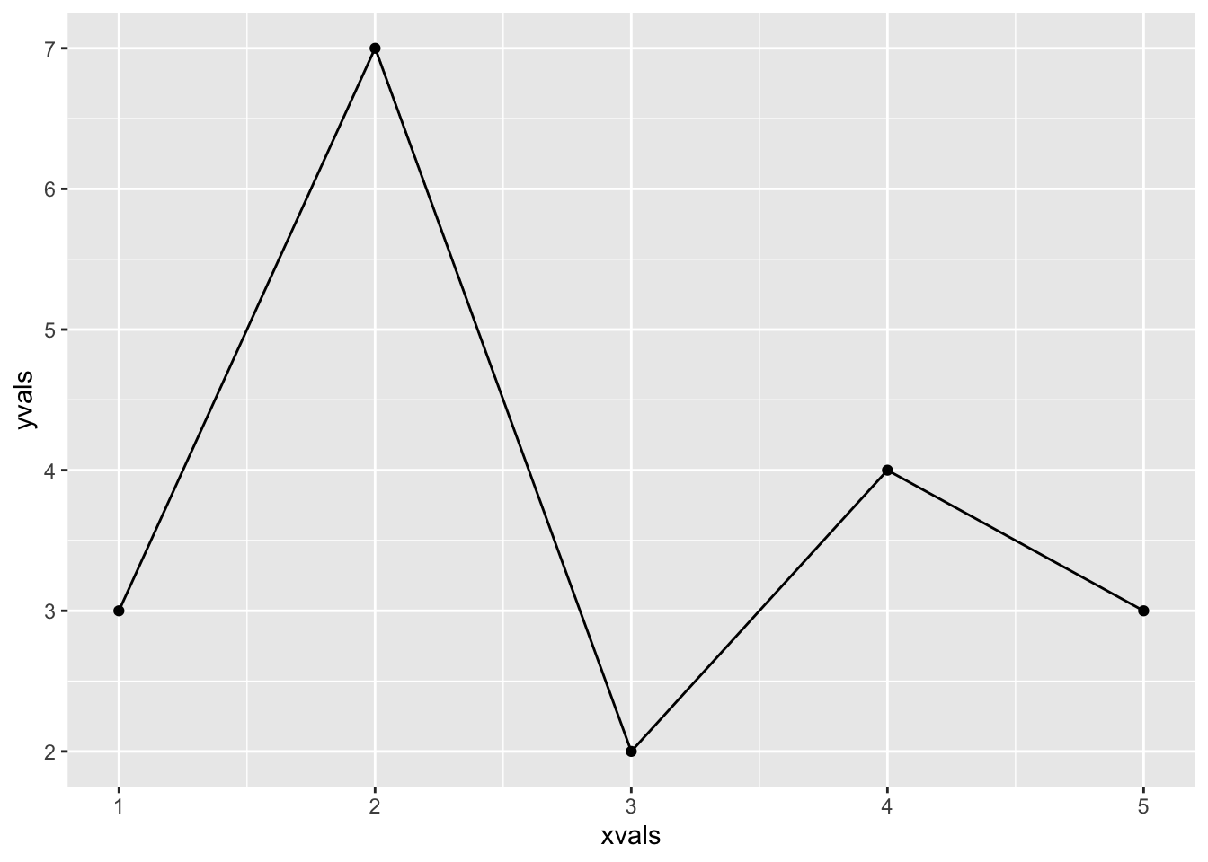

Figure 4.4: A ggplot2 plot with point and line geoms.

We’ll choose a scatterplot with connecting lines for our graph of the sequence. With a little more work we can get nice labels for the x and y-axes, and a title for the graph. Our collatz() function now looks like:

collatz <- function(n, limit = 10000) {
  # record initial number because we will change n
  initial <- n  
  numbers <- numeric(limit)
  counter <- 0
  while ( n > 1 & counter < limit) {
    counter <- counter + 1
    numbers[counter] <- n
    n <- collatzRule(n)
  }
  howMany <- min(counter, limit)
  steps <- 1:howMany
  cat("The Collatz sequence has ", howMany, " elements.\n", sep = "")
  show <- readline("Do you want to see it (y/n)?  ")
  if ( show == "y" ) {
    print(numbers[steps])
  }
  # use initial value to make plot title:
  plotTitle <- paste0("Collatz Sequence for n = ", initial)
  # make the plot
  ggplot(mapping = aes(x = steps, y = numbers[steps])) +
    geom_point() + geom_line() +
    labs( x = "Step", y = "Collatz Value at Step",
          title = plotTitle)
}

Try this version a few times, like so:

collatz(257)

It’s quite remarkable how much the sequence can rise and fall before hitting 1.

A further issue worth considering is that our collatz() function depends on the previously-defined function collatzRule(). In order for it to work correctly, R would need to be able to find the name collatzRule somewhere on the search path. If the user hasn’t already defined the collatzRule() function, then a call to `collatz() will fail.

One solution is simply to remind users of the need to define both collatzRule() and collatz() prior to running collatz(). Another solution—perhaps the kinder one—is to define the collatzRule() function in the body of collatz(). Let’s adopt this approach.

The final version of the collatz() function (with some validation thrown in for good measure) appears below.

collatz <- function(n, limit = 10000) {
  # add some validation:
  n <- suppressWarnings(as.integer(n))
  isValid <- !is.na(n) && n > 1
  if (!isValid ) {
    return(cat("Need an integer bigger than 1.  Try again."))
  }
  # define collatzRule:
  collatzRule <- function(m) {
    if ( m %% 2 == 0) {
      return(m/2)
    } else {
      return(3*m + 1)
    }
  }
  
  # On with the show!
  # Record initial number because we will change it:
  initial <- n 
  numbers <- numeric(limit)
  counter <- 0
  while ( n > 1 & counter < limit) {
    counter <- counter + 1
    numbers[counter] <- n
    n <- collatzRule(n)
  }
  howMany <- min(counter, limit)
  cat("The Collatz sequence has ", howMany, " elements.\n", sep = "")
  show <- readline("Do you want to see it (y/n)?  ")
  if ( show == "y" ) {
    print(numbers[1:howMany])
  }
  plotTitle <- paste0("Collatz Sequence for n = ", initial)
  steps <- 1:howMany
  ggplot(mapping = aes(x = steps, y = numbers[1:howMany])) +
    geom_point() + geom_line() +
    labs( x = "Step", y = "Collatz Value at Step",
          title = plotTitle)
}