6.7 Example: Dental Floss

If you are like me, you don’t like to run out of an item that you commonly use, so you always try to have a spare source for the item on hand. Take dental floss, for example. It’s difficult to know when the little box is almost out of floss. Hence I try to keep two boxes on hand in my bathroom drawer: the one I’m using, and a spare. The problem is that I can never tell which one is “the one I’m using” and which one is the spare. In fact on any given day I’m equally likely to pull a length of floss out of either one of the boxes.²¹

Let’s make the following assumptions:

A box of floss starts out with 150 feet of floss.
I start with two fresh boxes.
Every time I floss, each box has a 50% chance of being the box I pull from.
When I pull out floss, the length I choose to pull is a random number between 1 and 2 feet. If the box has less than than the amount I choose to pull, then:
- If the remaining length is more than 1 foot, I pull it all out and use it. (Next time I’ll have to use the other box.)
- If the remaining length is less than 1 foot, I also pull it all out, but I don’t use it because it’s not long enough. (I’ll have to move on to the other box.)

There are several interesting questions we could ask concerning this situation. In this example, let’s focus on finding the expected value of \(X\), the amount of floss left in the other box when I discover the one of the boxes is exhausted.

I would also like to get some idea of the distribution of \(X\)—the chance for it to assume each of its possible values. Unlike the previous “Number of Numbers” example, however, \(X\) is what we call a continuous random variable: it can assume any of the values in a range of real numbers. After all, the amount left in the “other” box could be anything from 0 to 150 feet: it could be 3.5633 feet or 5.21887 feet, or any real number at all, so long as it’s between 0 and 150. Although any real number value—3.5633 feet, for instance—is possible, it seems that the chance of \(X\) being exactly 3.5633 is vanishingly small, and the same goes for any of the possible real numbers value for \(X\). Hence it seems that the distribution of \(X\) cannot be described well with a table of the values that we actually get in a simulation: indeed, we are highly unlikely to get any value more than once in the course of our simulation.

One way to visualize the distribution of a continuous random variable is to make a density plot of a large, representative sample of its values. Let’s practice making a density plot for a random variable that R provides for us: a so-called normal random variable. Try this code:

x <- rnorm(100, mean = 70, sd = 3)

We have just asked R to produce 100 numbers chosen randomly from a normal distribution. The mean parameter sets what the values should be “on average,” and the sd parameter indicates how much they should typically differ from that average value. The bigger the sd, the bigger the difference between the mean and value actually obtained is liable to be.

Let’s get a look at the first ten values in the vector x:

x[1:10]

##  [1] 71.13092 70.90465 66.70593 66.60878 61.61040 72.16172 72.81736 69.31187 75.27739
## [10] 70.35210

Sure enough, the numbers are typically around the mean of 70, give or take 3 units or so.

We can use the ggplot2 package to produce a density curve from all 100 values in the vector x. (The resulting plot appears as Figure 6.2.)

library(ggplot2)

p <- ggplot(mapping = aes(x = x)) + geom_density() + geom_rug() +
  labs(x = "x-value")
p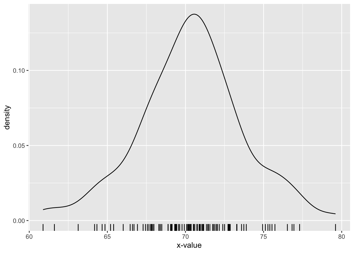

Figure 6.2: Density plot of 100 random values from a normal distribution with mean 70 and standard deviation 3.

The geom_density() part of the plotting-command produces the curve. The geom_rug() part produces tick-marks along the horizontal axis, each of which is located at a particular value in the vector x. You can see that the curve is higher where values are crowded together, and lower where the values are spread apart. The scale on the y-axis has been chosen carefully so that the area under the density curve between any two numbers \(a\) and \(b\) on the axis gives an estimate of the chance that the normal random variable would produce a value between \(a\) and \(b\). In this way the density curve gives us a visual sense of the distribution of the random variable: it seems rather likely to be between 67 and 73 (most of the area under the curve occurs there) and rather unlikely to be greater than 76, and so on.

We are now ready to simulate the dental-floss scenario. Since we have worked through the encapsulation-and-generalization development process a number of times by now, we will simply show a final-form implementation of a simulation function:

flossSim <- function(len = 150, min = 1, 
                     max = 2, reps = 10000, 
                     graph = FALSE, seed = NULL) {
  if ( !is.null(seed) ) {
    set.seed(seed)
  }
  
  # helper function to pick whihc box gets used:
  whichOne <- function(x) {
    if (x < 0.5 ) {
      return("a")
    } else return("b")
  }
  
  # vector to contains our results:
  leftover <- numeric(reps)
  
  # now the simulation.  Each time we loop through, we
  # start with two fresh boxes and use them until one of
  # them runs out.
  for (i in 1:reps ) {
    # set the initial lengh of the two fresh boxes:
    a <- b <- len
    
    # at the beignning, both can be used:
    bothOK <- TRUE
    
    # start flossing
    while ( bothOK ) {
      # determine which box is picked
      # < 0.5 is a; >= 0.5 is b;
      boxPicked <- whichOne(runif(1))
      
      # if we choose box a, attempt to use floss from it
      if ( boxPicked == "a" ) {
        if ( a < 1 ) {
          leftover[i] <- b
          bothOK <- FALSE
        } else {
          useAmount <- min(runif(1, min, max), a)
          a <- a - useAmount
          if (abs(a) < 10^(-4)) {
            leftover[i] <- b
            bothOK <- FALSE
          }
        }
      }
      
      # use floss from b (if we choose it) 
      if ( boxPicked == "b" ) {
        if ( b < 1 ) {
          leftover[i] <- a
          bothOK <- FALSE
        } else {
          useAmount <- min(runif(1, min, max), b)
          b <- b - useAmount
          if (abs(b) < 10^(-4)) {
            leftover[i] <- a
            bothOK <- FALSE
          }
        }
      }
        
    }  # end while  loop
  }    # end for loop
  
  # report results:
  if ( graph ) {
    plotTitle <- paste0("Dental-Floss Simulation with ", reps, " Repetitions")
    p <- ggplot(mapping = aes(leftover)) + geom_density() +
      labs(x = "Amount left in spare (ft)",
          title = plotTitle)
    # add a rug of individual points, provided there are not too many:
    if ( reps <= 100 ) {
      p <- p + geom_rug()
    }
  }
  print(p)
  cat("The average amount left in the spare is:  ", 
      mean(leftover), ".", sep = "")
}      # end flossSim

Let’s give it a try with one thousand repetitions.

flossSim(reps = 1000, graph = TRUE, seed = 3535)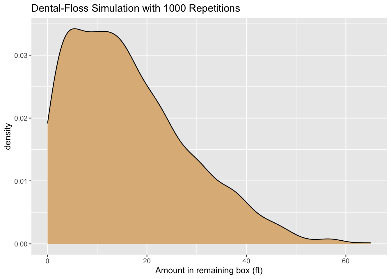

Figure 6.3: Density plot of the results of a dental-floss simulation.

## The average amount left in the spare is:  16.55715.

A density plot of the results appears as Figure 6.3. The expected value of the amount left in the remaining box is about 16.3 feet, but you can see from the plot that there is quite a bit of variability: it’s not all that unlikely to have 40 or more feet left!

A scenario similar to this one is discussed in (J.Nahin 2008), see p. 52.↩︎