5 Turtle Graphics

Figure 5.1: Turtles, by xkcd.

In this chapter we will practice our knowledge of R—and of basic programming concepts—in the context of a special R-package for graphics: package TurtleGraphics (Cena et al. 2018). Many of the examples from this Chapter are drawn from the Vignette for the package.¹⁴

5.1 Basic Movements

First, we begin by loading the package:

library(TurtleGraphics)

In order to create a Turtle Graphics scenario, call the function turtle_init(). You get the plot shown in Figure 5.2.

turtle_init()

Figure 5.2: Initialized Turtle

By default the turtle is positioned in the middle of a square of dimensions 100 units by 100 units. (These dimensions can be changed, as we will see later on.)

You can get the turtle’s position at any time:

turtle_getpos()

##  x  y 
## 50 50

The turtle also begins facing North. This is considered to be angle 0, as you can tell by asking for the current angle of the turtle:

turtle_getangle()

## angle 
##     0

Now let’s make the turtle move. If you are following along on your own computer, it’s best to run the lines of code one at a time, so you can see the effect of each command. (If you run multiples lines, you’ll only see the graph produced by the final line.)

turtle_forward(dist = 30)
turtle_backward(dist = 10)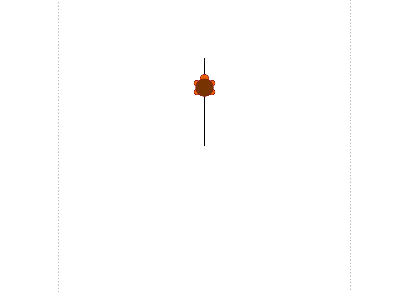

Figure 5.3: First Movements

The result appears in Figure 5.3. Next we’ll add a little triangle:

turtle_right(90)
turtle_forward(10)
turtle_left(angle = 135)
turtle_forward(14.14)
turtle_left(angle = 90)
turtle_forward(14.14)
turtle_left(angle = 135)
turtle_forward(10)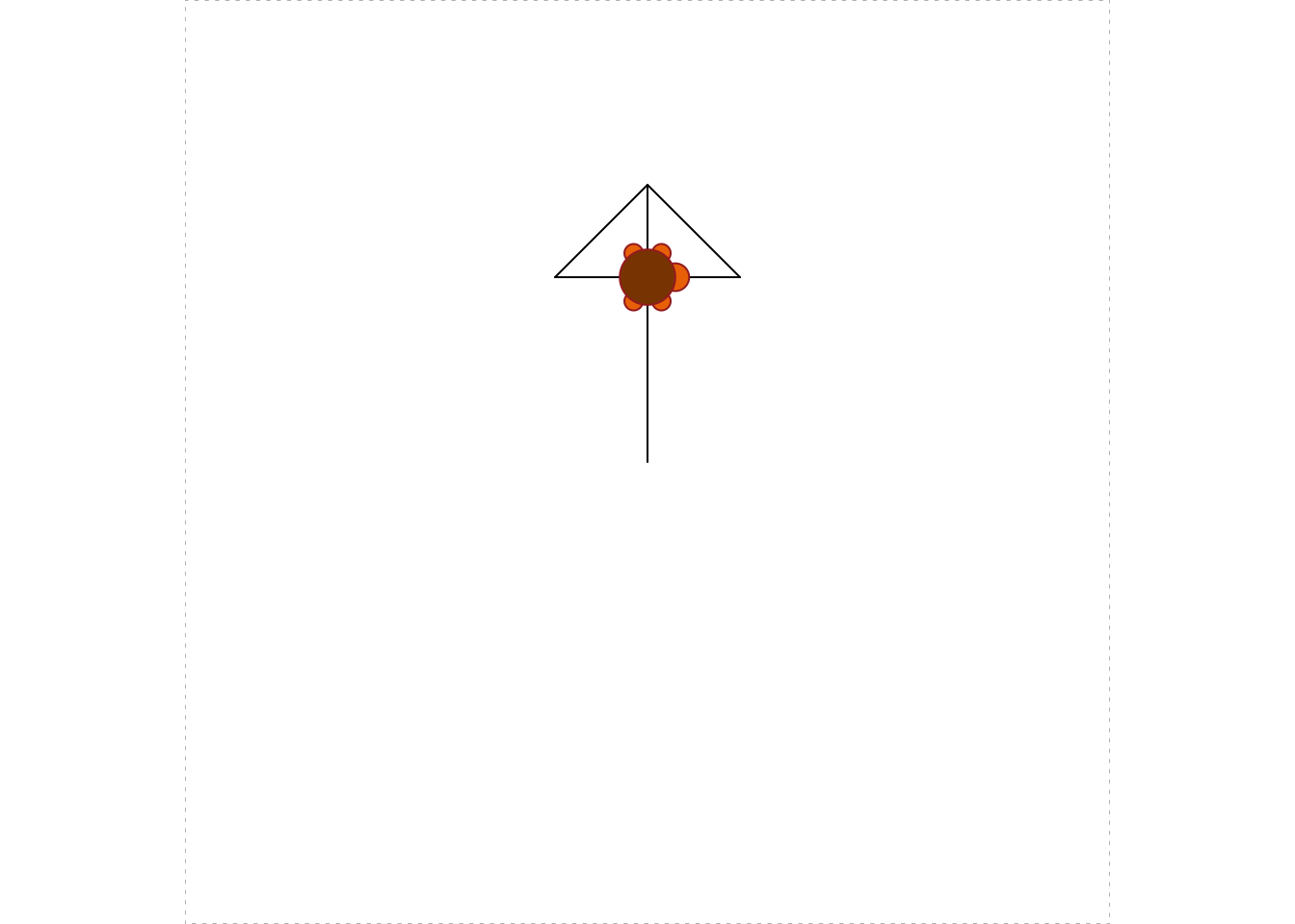

Figure 5.4: Adding a Triangle

You can see the triangle in Figure 5.4.

The turtle is set in the “down” position, so that it leaves a trace out the path that it follows. You can avoid the trace by pulling the turtle “up” with turtle_up(). Whenever you want to restore the tracing, call turtle_down(). See Figure 5.5 for the results of the following code.

turtle_up()  # stop tracing
turtle_right(angle = 90)
turtle_forward(dist = 10)
turtle_right(angle = 90)
turtle_forward(dist = 17)
turtle_down()  # start tracing again
turtle_left(angle = 180)
turtle_forward(dist = 34)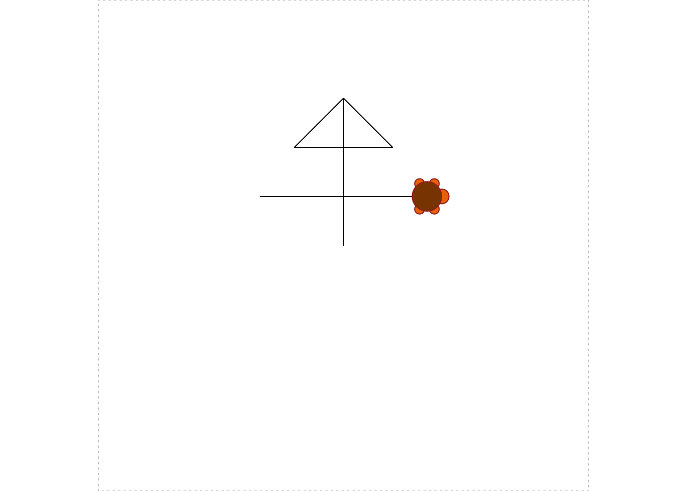

Figure 5.5: We moved the turtle around in the up position, then put the turtle down and traced out a line segment.

You can change the color of the lines your turtle draws:

turtle_col(col = "green")

In R here are many, many colors to choose from, and 657 of them even have names. To view them, use the colors() function:

colors()

You can also hide your turtle, and show it again any time you like. See Figure 5.6 for the results of the following code.

turtle_hide()
turtle_left(angle = 150)
turtle_forward(dist = 20)
turtle_left(angle = 60)
turtle_forward(dist = 20)
turtle_show()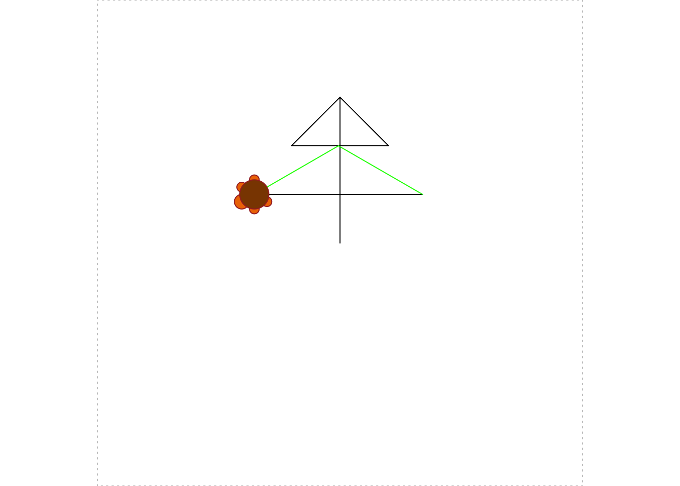

Figure 5.6: The graph after hiding, moving and showing.

Finally, you can choose the type of line your turtle draws, and the width of the line. See Figure 5.7 for the results of the following code.

turtle_left(angle = 150)
turtle_lty(lty = 4)
turtle_forward(dist = 17)
turtle_lwd(lwd = 3)
turtle_forward(dist = 15)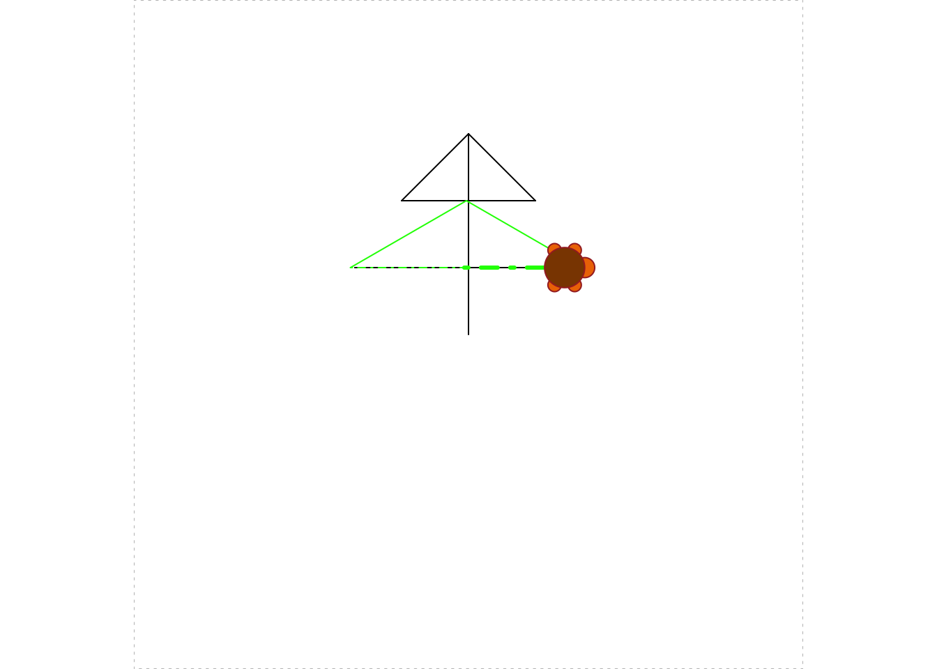

Figure 5.7: Choosing line-type and line-width.

Note: you can learn more about lty and lwd with help(par).

5.2 Making Many Movements: An Introduction to Looping

Eventually we want to make some complex figures that require many movements on the part of the turtle. In order to make these go faster, we can turn off some of the turtle graphing by wrapping the desired movements in turtle_do(). See Figure 5.8 for the results of the following code.

turtle_init()
turtle_do({
  turtle_move(10)
  turtle_turn(45)
  turtle_move(15)
})

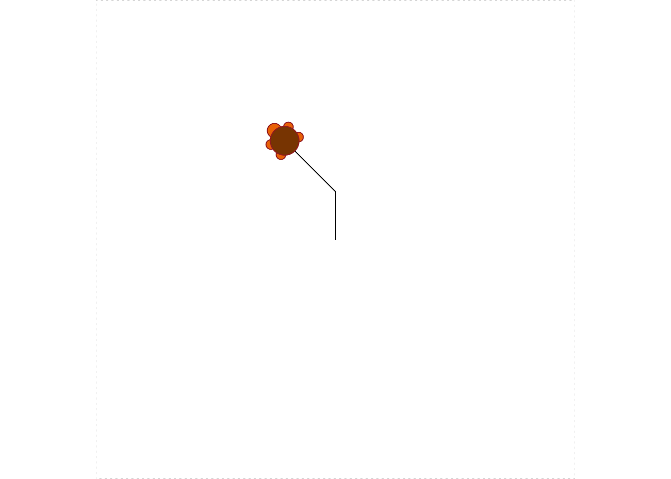
Figure 5.8: After final movement.

(turtle_turn() turns to the left by default.) Of course, for such a small number of movements using turtle_do() does not matter much, but we will practice using it for a bit.

How might we make a square? The following code offers one way to do it. See Figure 5.9 for the results.

turtle_init()
turtle_do({
  turtle_move(20)
  turtle_right(90)
  turtle_move(20)
  turtle_right(90)
  turtle_move(20)
  turtle_right(90)
  turtle_move(20)
  turtle_right(90)
})

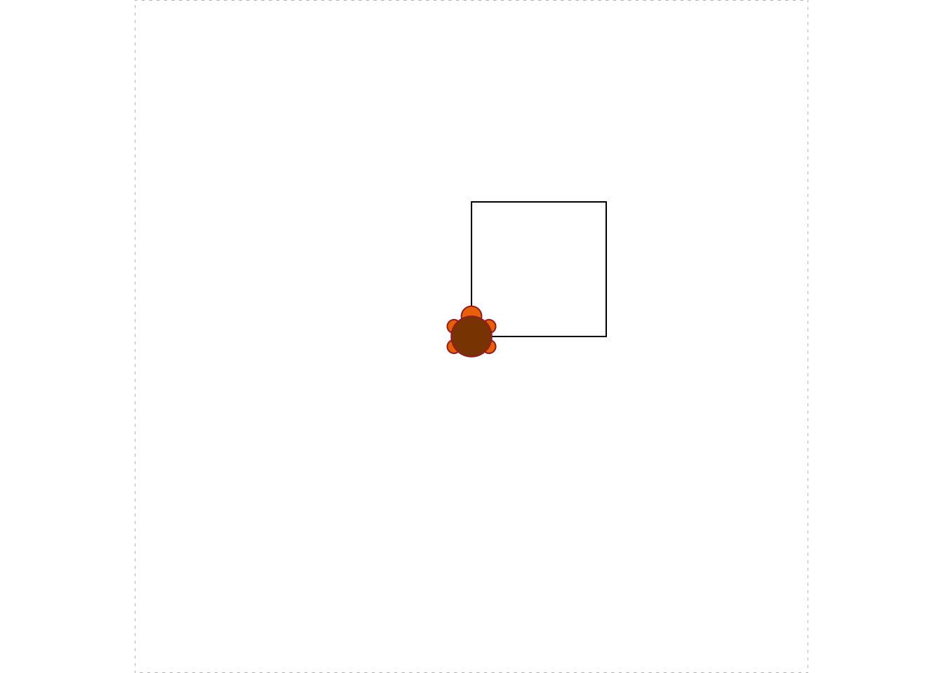
Figure 5.9: Making a square.

This is a bit repetitious. Surely we can take advantage of the fact that there is a clear pattern to the turtle’s movements. A for-loop seems called for, as in the following code to build the square:

turtle_init()
turtle_do({
  for(i in 1:4) {
    turtle_forward(dist = 20)
    turtle_right(angle = 90)
  }
})

As we learned in Chapter 4, the more you need to repeat a particular pattern, the more it makes sense to write your code with a loop. Suppose, for example, that you decide to make regular octagons. A regular octagon has eight sides, and you turn 45 degrees after drawing each side. You can do this easily by modifying the square-code as follows (see Figure 5.10 for the results):

turtle_init()
turtle_do({
  for(i in 1:8) {
    turtle_forward(dist = 20)
    turtle_right(angle = 45)
  }
})

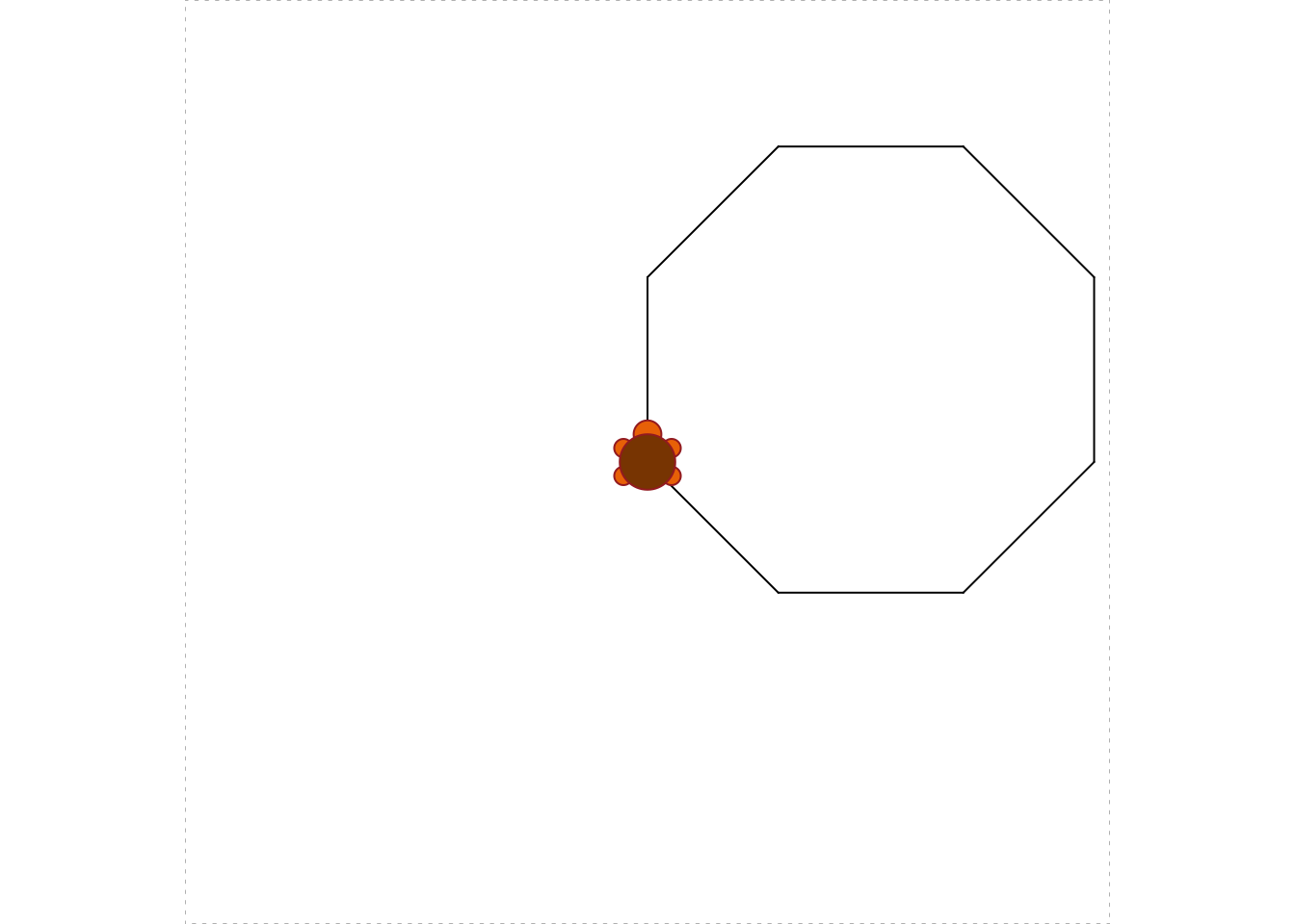
Figure 5.10: Making an octagon.

You can even make many small turns, so that the resulting figure starts to look like a circle (see Figure 5.11 for the results):

turtle_init()
turtle_setpos(x = 30, y = 50)
turtle_do({
  for(i in 1:180) {
    turtle_forward(dist = 1)
    turtle_right(angle = 2)
  }
})

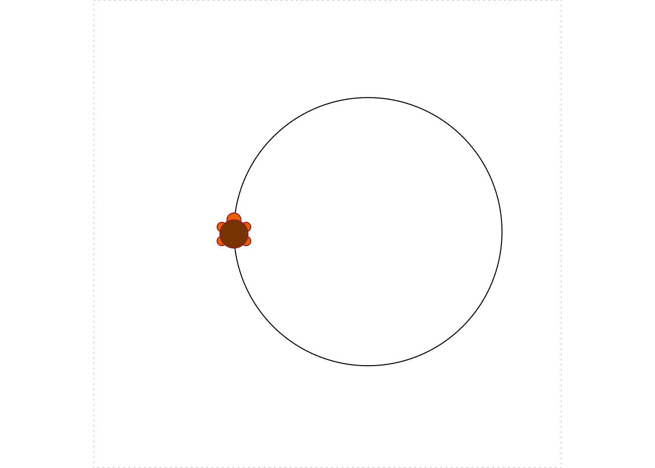
Figure 5.11: Making a circle.

Notice that in the above code the turtle was initially set a bit to the left of center, so that the resulting circle would be situated close to middle of the region.

If you allow the index variable to be involved in the computations in the body of the loop then you can start making more complex figures. For example, here is the code for a spiral (see Figure 5.12 for the results):

turtle_init(width = 150, height = 150, mode = "clip")
turtle_do({
  turtle_right(90)
  for (i in 1:720) {
    turtle_left(1)
    turtle_forward(i/720)
  }
})

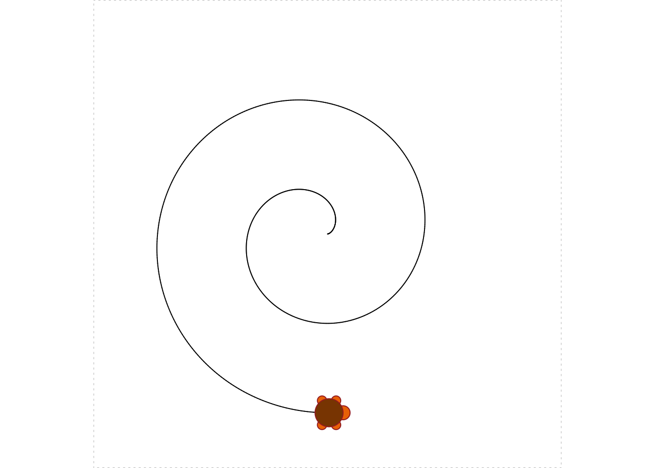
Figure 5.12: Using a loop to make a spiral.

The turtle turns one degree every time R goes through the loop, but the amount it travels forward (\(i/720\)) increases as the index variable i increases.

Another thing to notice is that we set the width and height of the region ourselves, so that the spiral would fit into it. We also set mode to clip rather then leaving it at its default value of error. With mode = "clip", R won’t throw an error message at you when the turtle moves outside of its region. Clip-mode is very handy when you are developing a graph and don’t know in advance precisely where the turtle will go.

5.2.1 Practice Exercises

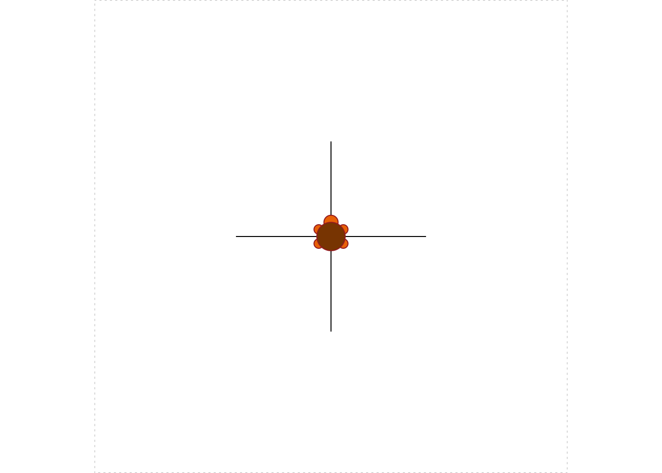
Write a program to make a four-sided star with rays of length 20 each, like this:
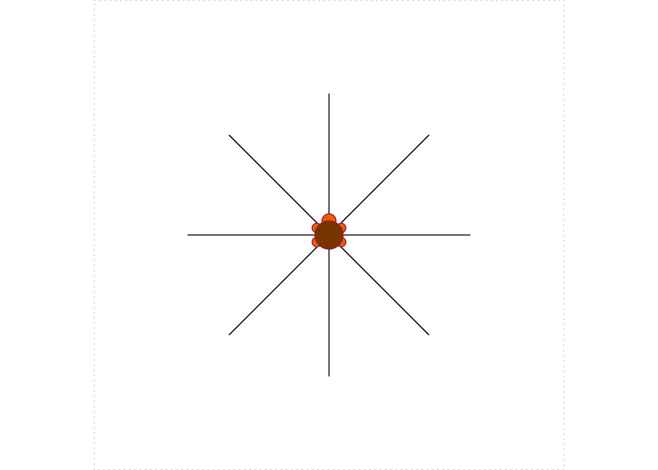
Write a program to make an eight-sided star with rays of length 30 each, like this:

5.2.2 Solutions to the Practice Exercises

In order to make a single ray you walk 20 units forward from a central point, then walk 20 units back to the center. In order to prepare to make the next ray, you turn after you get back to the center. Since you plan on four rays, you must turn \(360/4 = 90\) degrees each time. It makes sense to trace each ray once inside a for-loop. Using turtle_do() will make the loop run much faster. Here’s the code:
```
turtle_init(mode = "clip")
turtle_do({
  for ( i in 1:4 ) {
    turtle_forward(20)
    turtle_backward(20)
    turtle_left(90)
  }
})
```
This time in order to make a single ray you walk 30 units forward from a central point, then walk 30 units back to the center. Since you now plan on eight rays, you must turn \(360/8 = 45\) degrees each time. Again it makes sense to trace each ray once inside a for-loop. Here’s the code:
```
turtle_init(mode = "clip")
turtle_do({
  for ( i in 1:8 ) {
    turtle_forward(30)
    turtle_backward(30)
    turtle_left(45)
  }
})
```

5.3 Writing Turtle Functions

Once you have designed some shapes that you think you might want to draw again, you should write them up as functions. Here for example, is the code for a function that makes squares:

turtle_square <- function(side) { 
  turtle_do({
    for (i in 1:4) {
      turtle_forward(side)
      turtle_right(90)
    }
  })
}

Note that the user can vary the length of a side. You would use it like this:

turtle_init(mode = "clip")
turtle_square(side = 30)

5.3.1 Practice Exercises

Write a function called star8() that makes an eight-sided star with rays of length 20 each. The user should be able to specify the thickness of the rays (think turtle_lwd()). The body of the function should begin with turtle_init() so that the star is always drawn inside a new field. The function should take a single parameter called width, the desired thickness of the rays. Typical examples of use should be as follows:
```
star8(width = 2)
```
```
star8(width = 10)
```
Modify your star8() function to make a new function called superstar8() that takes an additional parameter called color that allows the user to specify the color of the rays. The default value of color should be "burlywood". Typical examples of use should be as follows:
```
superstar8(width = 5)
```
```
superstar8(width = 15, color = "lavenderblush4")
```

5.3.2 Solutions to the Practice Exercises

From the Practice Exercises of the previous section we are already familiar with making 8-ray stars; we just need to encapsulate the process into a function. Here’s the code:

star8 <- function(width) {
  turtle_init(mode = "clip")
  turtle_lwd(lwd = width)
  turtle_do({
  for ( i in 1:8 ) {
    turtle_forward(20)
    turtle_backward(20)
    turtle_turn(45)
  }
  })
}

Try this:

superstar8 <- function(width, color = "burlywood") {
  turtle_init(mode = "clip")
  turtle_lwd(lwd = width)
  turtle_col(col = color)
  turtle_do({
  for ( i in 1:8 ) {
    turtle_forward(20)
    turtle_backward(20)
    turtle_turn(45)
  }
  })
}

5.4 Random Moves

So far our turtle has moved in very regular and disciplined ways. It’s time to break the pattern, a bit. R has a quite a few functions to generate numbers that look “random”; we will use some of these functions to make the turtle move about randomly.

5.4.1 Sampling from a Vector

You have already met the sample() function (see Section 4.2.1). Let’s take a closer look at it.

sample() makes a random choice from a given vector. From the R-help we read that the general form of a call to sample is as follows:

sample(x, size, replace = FALSE, prob = NULL)

In the above call:

x is the vector from which we wish to sample (R refers to it as the “population”);
size is the number of random samples we want;
replace says whether or not to replace each member of the population after we have sampled it.
prob specifies the desired probability for each member of the population to be chosen. If it is left at its default value of NULL, then each element of the vector has the same chance to be chosen.

A few examples will help us understand how the arguments work:

vec <- 1:10 # we'll sample from this vector
sample(vec, 1)

## [1] 7

We got only one number because we set size to 1. Every element in vec had an equal chance of being the element selected. This time we got 7, but if you were to run the function again for yourself your results would probably be different.

Let’s sample 10 numbers from vec:

sample(vec, 10)

##  [1]  1  9 10  5  4  3  2  7  8  6

Because replace was left at its default value of FALSE, R did not replace numbers after pulling them from the vec. After each sample, the remaining numbers all had the same chance to be picked next. Setting size to the length of x and keeping replace = FALSE therefore has the effect of randomly shuffling the elements of x.

Of course when replace = FALSE any attempt to sample more than the number of elements of vec will result in an error:

sample(vec, 11)

Error in sample.int(length(x), size, replace, prob) : 
cannot take a sample larger than the 
population when 'replace = FALSE'

When we set replace = TRUE then each selected element is returned to the population. At any stage, the chance for a given member of the population to be the one selected next is the same—no matter how many times that member has already been selected. Thus, when replace = TRUE you are liable to see repeats:

sample(vec, 20, replace = TRUE)

##  [1]  5  3  5  5  8  8  9 10  5  9  4  5  6  4 10  7  1  8  3  5

When the prob parameter is left at its NULL value, R gives each member of the population the same chance to be the member that is selected. It is possible to adjust the probabilities of selection by setting prob to a vector of probabilities (one for each corresponding member of x). Thus, suppose we want to select 20 numbers from vec, according to the following the probabilities:

5% chance of selection, for each number from 1 to 8;
30% chance for 9 to be selected;
30% chance for 10 to be selected.

Then we can call sample() like this:

sample(vec, 20, replace = TRUE,
       prob  = c(rep(0.05, 8), 0.30, 0.30))

##  [1]  9  1  9 10  9  6  8  9  4  7 10 10  9  2  6  9  5  9 10 10

Notice the majority of 9’s and 10’s: this was fairly likely to occur since each selection had a 60% chance of turning out to be 9 or 10.

5.4.2 Application: a Bouncing Turtle

Let’s apply sample() to design a scenario in which the turtle moves a fixed amount at each step, but the direction—north, east, south, or west—is completely random. When the turtle reaches the boundary of its domain, however, we would like it to “bounce back”: i.e., take a step in the direction opposite to the step that brought it to the boundary. We will also query the user prior to each step, asking if he/she wants to see another move. This not only allows the user to decide when to end the scenario; it also permits the user to see where the turtle is after each step.

One possible implementation is as follows:

turtle_bounce <- function(side = 60, step= 10) {
  if ( (side/2) %% step != 0 ) {
    stop("Side-length divided by two must be a multiple of step.")
  }
  bounds <- c(0, side)
  turtle_init(side, side, mode = "clip")
  origin <- turtle_getpos()
  cp <- turtle_getpos()
  repeat {
    move <- readline(prompt = "Go Again? (enter q to quit):  ")
    if ( move == "q") break
    x <- cp["x"]
    y <- cp["y"]
    if (x %in% bounds | y %in% bounds) {
      angle <- 180
    } else {
      angle <- sample(c(0,90,180,270), 1)
    }
    turtle_right(angle)
    turtle_forward(step)
    cp <- round(turtle_getpos(), 0)
    print(cp)
  }
  cat("All done!")
}

Play the game a few times, to get a feel for how it works:

turtle_bounce(60, 15)

Let’s examine the code a bit more closely.

The definition indicates that there are two parameters: side and step.

The side parameter gives the dimensions of the Turtle’s field. Thus if side were set to 60—which is the default—then the field would be a 60-by-60 square, with the origin \((0,0)\) in at lower-left corner and the point \((60, 60)\) at the upper-right corner. When the turtle is initialized it will appear in the middle of the square, at the point \((30, 30)\).
step specifies how many units the turtle will move at each step. In this analysis we will assume that step is set to 15.

Inside the function, we begin with a bit of input-validation:

if ( (side/2) %% step != 0 ) {
    stop("Side-length divided by two must be a multiple of step.")
  }

Remember that the turtle will start at \((\texttt{side}/2, \texttt{side}/2)\) and will move step each time. If \(\texttt{side}/2\) is not evenly divisible by step then the turtle would be able to go from inside its field to outside in a single step. We don’t want that to happen so we stop the user if the remainder after dividing \(\texttt{side}/2\) by side is anything other than zero.

If the input is OK, then we set up a vector bounds that records the smallest and largest possible values for the \(x\) and \(y\) coordinates of the turtle:

bounds <- c(0, side)

Next, we initialize the turtle in the middle of the field and record its initial position in the vector cp:

turtle_init(side, side, mode = "clip")
origin <- turtle_getpos()
cp <- turtle_getpos()

(You can think of cp as short for: “current position”.)

Next, we enter a repeat-loop. Inside the loop we begin with:

move <- readline(prompt = "Go Again? (enter q to quit):  ")
if ( move == "q") break
x <- cp["x"]
y <- cp["y"]

We first asked the user if she wanted to quit. If she enters “q” then we’ll break out of the loop and end the scenario. If she enters anything else (including just pressing Enter) then we record the \(x\) and \(y\) coordinates of the turtle’s current position in the vectors x and y respectively.

Our next task is to determine how the turtle should move:

if (x %in% bounds | y %in% bounds) {
      angle <- 180
    } else {
      angle <- sample(c(0,90,180,270), 1)
    }

If the turtle is at a boundary (either x equal to 0 or 60 or y equal to 0 or 60) then we need to “bounce back”. This corresponds to making the turtle turn right by 180 degrees and then step. On the other hand if the turtle is not at a boundary then the direction of the turtle should be random, so we should have it turn right by either 0, 90, 180 or 270 degrees, with each possibility being equally likely. This is accomplished with the above call to the sample() function.

Having determined the amount by which to turn prior to the next step, we then have the turtle turn that amount and take the step:

turtle_right(angle)
turtle_forward(step)

Finally, we set cp to the new position of the turtle, and print that position out to the console for the user to see:

cp <- round(turtle_getpos(), 0)
print(cp)

Note that we rounded off the position to the nearest while number. This was done because the authors of the TurtleGraphics package use floating point arithmetic for their numerical operations, so sometimes the computed positions differ from whole numbers by a very tiny amount.

We then repeat the loop.

5.4.3 Uniform Random Numbers.

sample() picks an element from a finite population. Sometimes, though, we want R to give the impression that it has picked a real number at random out of a range of real numbers. This can be accomplished with the runif() function.

A call to runif() looks like this:

runif(n, min = 0, max = 1)

The idea is that R will produce n real numbers that have the appearance of having been drawn randomly from the interval of real numbers whose lower and upper bounds are specified respectively by min and max.

Thus, to get 10 “random” numbers that all lie between 0 and 1, you can leave min and max at their defaults and ask for:

runif(10)

##  [1] 0.646902839 0.394225758 0.618501814 0.476891136 0.136097186 0.067384386 0.129152617
##  [8] 0.393117930 0.002582699 0.620205954

5.4.4 Pseudo-Randomness and Setting a Seed

It’s important to point out that R doesn’t generate truly random numbers.¹⁵ After all, R simply runs a computer which operates according to a set of completely-specified steps. Thus the random data generated by R and by other computer languages is often called pseudorandom. Although the functions for random-number generation have been carefully designed so as to follow many of the statistical laws we associate with randomness in nature, all of the pseudo-random output is determined by an initial value and a deterministic number-generating algorithm.

We actually have the ability to set the pseudorandom data ourselves. This is called setting the random seed. From any specified seed, the result of calls to R’s random-data functions will be completely determined (although—just as in the case of “real” randomness—the output will still probably “look” random).

The set.seed() function will fix the random output. Try running the following two lines of code more than once:

set.seed(2025)
runif(10)

##  [1] 0.7326202 0.4757614 0.5142159 0.4984323 0.7802845 0.5042522 0.8984003 0.1278527
##  [9] 0.6446721 0.5695311

You will get the same output every time. If you change the argument of set.seed() to some other integer the output will probably change—but it will stay the same when you run the code again from that that new seed.

5.4.5 Application: a Drunken Turtle

We will now modify the previous scenario so that the turtle’s motion will be almost completely random. Even though it will take the same-size step every time, the angle at which it steps will be completely random: any real number of degrees from 0 to 360. We will also show the user the position of the turtle at each step, and use the “distance formula” from high-school geometry to compute and display the current distance of the turtle from the place where it started.

turtle_drunk <- function(side, step) {
  turtle_init(side, side, mode = "clip")
  # save (side/2, side/2), the turtle's initial position:
  initial <- turtle_getpos()
  repeat {
    move <- readline(prompt = "Go Again? (enter q to quit):  ")
    if ( move == "q") break
    # pick a random angle to turn by:
    angle <- runif(1, min = 0, max = 360)
    turtle_left(angle)
    turtle_forward(step)
    # get new position, make it the current position:
    cp <- turtle_getpos()
    # print to console:
    print(cp)
    # determine distance from initial position (round to 3 decimals):
    distance <- round(sqrt((cp[1] - initial[1])^2 + (cp[2] - initial[2])^2),3)
    # prepare message to console,and print it:
    message <- paste0("Distance from starting point is: ", distance)
    cat(message)
  }
  cat("All done!")
}

Try the game once or twice:

turtle_drunk(100, 5)

It is natural to wonder how likely the turtle is to wander back close to where it started, and to wonder how often that will happen. We will address questions like these in Chapter 6.

5.4.6 Practice Exercises

Many of these exercises don’t deal directly with turtles, but instead drill you on the sample() and runif()` functions.

Write a call to the sample() function so that it will pick a whole number at random from 1 to 10. Each number should have the same chance to be selected.
You have a large bag of M&Ms. You reach in an grab a few. You have an equal to chance to grab any number of M&Ms from 1 to 10. (You can’t grab more than 10, and you can’t grab none.) Write a one-line command that expresses how many you grab.
Write a call to the sample() function that will pick five numbers at random from the whole numbers from 1 to 10. On each pick, each of the ten numbers should have a 1-in-10 chance to be selected.
Write a call to the sample() function that will pick five numbers at random from the whole numbers from 1 to 10. It should not be possible to get the same number twice.
Write a call to the sample() function that scrambles the whole numbers from 1 to 10 in a random order.
Write a call to the sample() functions that randomly re-orders the lowercase letters of the English alphabet.
The function color() produces a character vector of the named colors that R is prepared to draw. Run it at the Console:
```
colors()
```
How many named colors are there? Let’s let R find out for us:
```
length(colors())
```
```
## [1] 657
```
Write a call to the sample() function that will pick a single named color at random.
Write a call to runif() that will produce a single random real number between 0 and 1.
Write a call to runif() that will produce 20 random real numbers between 0 and 1.
Write a call to runif() that will produce 30 random real numbers, each of them between 10 and 15.
You enter a forest where there are many sticks on the ground. Each of them is equally likely to be anywhere between 0 and 10 feet long. You pick up five sticks at random. Write a one-line R-command that produces the length of shortest stick that you pick up.
Write a function called randomColor8() that produces an 8-ray star. Here are the specs:
- The user should be able to determine the type of the line (think turtle_lty()).
- Each ray should have a 30% chance of being red and a 70% chance of being blue.
- In addition, the length of each ray should be a random real number between 10 and 40.
- The function should take a single parameter called type that the user can set to determine the line-type for the rays; its default-value should be 1.
- The width of each ray should be 5.
Typical examples of use should be as follows:
```
randomColor8()
```
```
randomColor8(type = 3)
```

5.4.7 Solutions to the Practice Exercises

sample(1:10, size = 1)
The previous function call will do: sample(1:10, size = 1).
sample(1:10, size = 5, replace = TRUE)
sample(1:10, size = 5, replace = FALSE)
sample(1:10, size = 10, replace = FALSE)
sample(letters, size = length(letters), replace = FALSE)
sample(colors(), size = 1)
runif()
runif(20)
runif(30, min = 10, max = 15)
min(runif(5, min = 0, max = 10))

Try this:

randomColor8 <- function(type = 1) {
  allowedColors <- c("red", "blue")
  turtle_init(mode = "clip")
  turtle_lty(lty = type)
  turtle_lwd(lwd = 5)
  turtle_do({
    for ( i in 1:8 ) {
      turtle_col(col = sample(allowedColors, 
                              size = 1, 
                              prob = c(0.3, 0.7)))
      rayLength <- runif(1, min = 10, max = 40)
      turtle_forward(rayLength)
      turtle_backward(rayLength)
      turtle_left(45)
    }
  })
}

5.5 More Complex Turtle Graphs

Simple instructions, when combined with looping, can produce quite complex patterns. Consider the following process (with results shown in Figure 5.13):

turtle_init(1000, 1000, mode = "clip")
turtle_do({
  turtle_setpos(600,400)
  turtle_right(90)
  for (i in 1:2000) {
    turtle_right(i)
    turtle_forward(sqrt(i))
  }
})

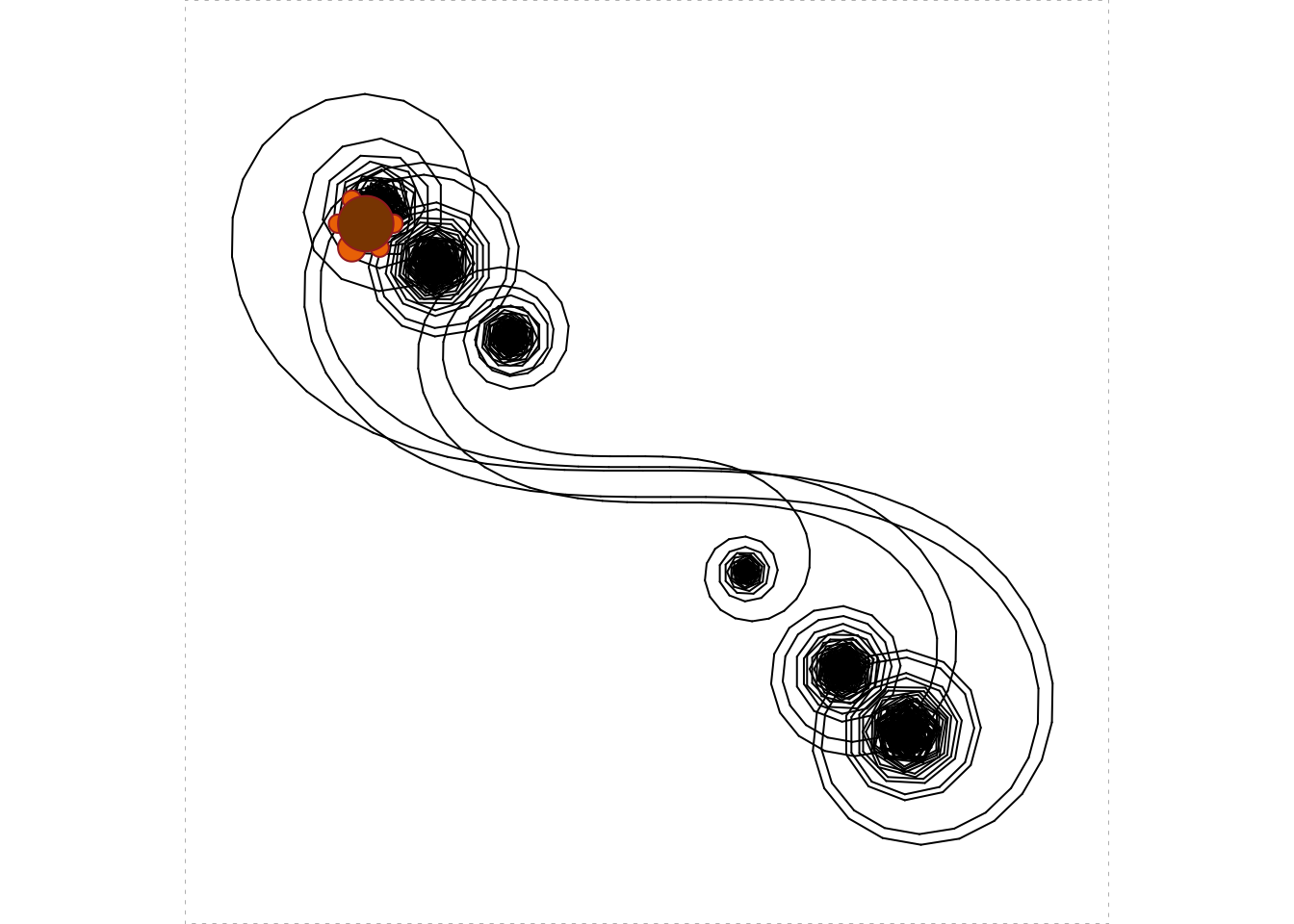
Figure 5.13: Galactic Zany!

You might enjoy figuring out why this pattern occurs. As you ponder this, it might help to construct a set of “ragged” spirals with somewhat larger steps, and pause at each step. Code like the following might be useful:¹⁶

turtle_init(1000, 1000, mode = "clip")
turtle_do({
  i <- 1
  turtle_right(90)
  repeat {
    bidding <- readline("Proceed? (Enter q to quit) ")
    if ( bidding == "q") break
    turtle_right(i)
    turtle_forward(2*sqrt(i))
    cat(paste0("Turned ", i, " degrees,\n"))
    cat(paste0("stepped forward ", round(2*sqrt(i), 3), " units.\n"))
    cat("Turtle's current angle is: ", turtle_getangle(), " degrees.\n")
    i <- i + 20
  }
  cat("All done!")
})

5.6 Artistic Turtles

In the Practice Exercises (see Section 5.4.6) you met the colors() function. Let’s have the Turtle put it to good use.

First of all, we might ask the Turtle to show us a sample of a given color:

turtle_show_color <- function(color) {
  cat("I'm drawing a ", color, " square!", sep = "")
  turtle_init()
  turtle_col(color)
  turtle_lwd(50)
  turtle_do({
    turtle_setpos(x = 30, y = 30)
    turtle_square(40)
  })
}

Note the very thick lines specified above: turtle_lwd(50). Our turtle will draw a square with very thick sides that have the desired color. Let’s ask for burlywood. The resulting color-swatch is shown in Figure 5.14.

turtle_show_color("burlywood")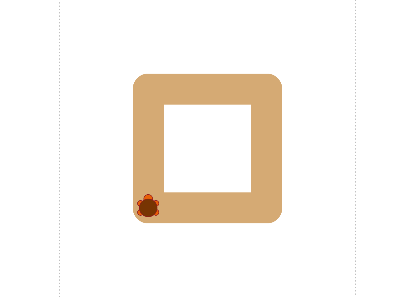

Figure 5.14: I’m drawing a burlywood square!

Feel free to ask for a random color. The result of the call below is shown in Figure 5.15.

turtle_show_color(sample(colors(), size = 1))

Figure 5.15: I’m drawing a palegreen2 square!

The function below is the Turtle’s attempt to dash off a quick imitation of the work of Jackson Pollack, the great American abstract expressionist:

turtle_quick_pollack <- function(strokes) {
  turtle_init(mode = "clip")
  turtle_lwd(50)
  colorsUsed <- character(strokes)
  turtle_do({
    for ( i in 1:strokes ) {
      randomColor <- sample(colors(), size = 1)
      turtle_col(randomColor)
      colorsUsed[i] <- randomColor
      randomAngle <- runif(1, min = 0, max = 360)
      turtle_left(randomAngle)
      turtle_forward(10)
    }
  })
  cat("Behold my masterpiece!  It was painted with:\n")
  print(colorsUsed)
}

Note that the colors used are output to the console. Let’s have it make a picture with 50 strokes made by random-colored brushes. The resulting painting appears as Figure 5.16

turtle_quick_pollack(50)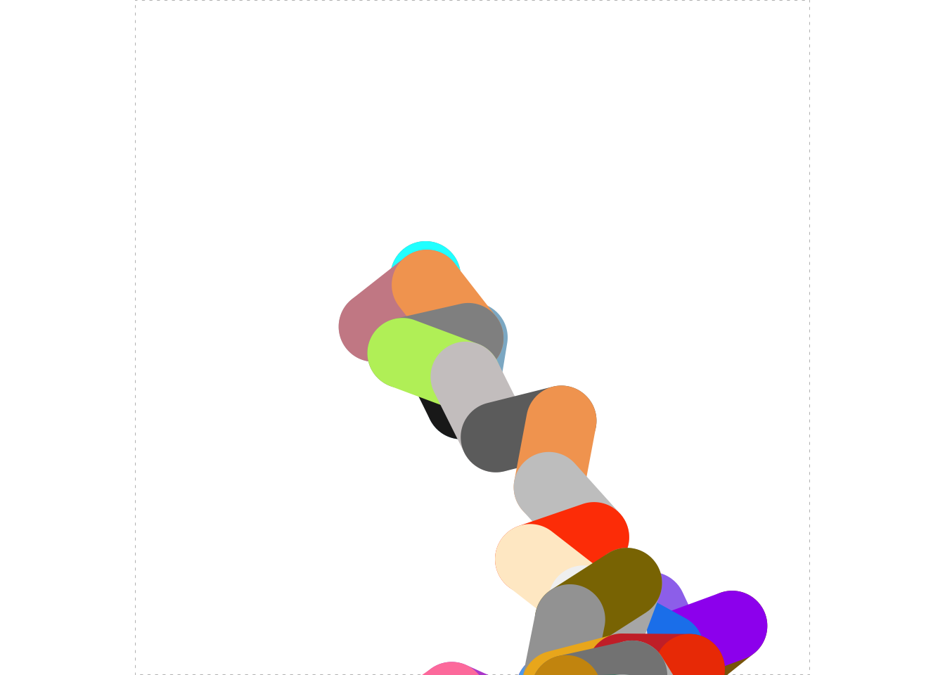

Figure 5.16: Behold my masterpiece!

## Behold my masterpiece!  It was painted with:
##  [1] "lightskyblue3"   "gray12"          "grey62"          "cyan"           
##  [5] "gray77"          "lightpink3"      "sandybrown"      "gray57"         
##  [9] "darkolivegreen2" "snow3"           "grey43"          "sandybrown"     
## [13] "grey79"          "orangered1"      "blanchedalmond"  "gray95"         
## [17] "mediumpurple2"   "darkgoldenrod4"  "purple"          "dodgerblue2"    
## [21] "grey93"          "violetred"       "steelblue2"      "grey71"         
## [25] "gold4"           "grey64"          "goldenrod2"      "brown3"         
## [29] "orangered2"      "gray"            "gray52"          "darkgoldenrod3" 
## [33] "grey70"          "lightslategrey"  "aquamarine4"     "grey71"         
## [37] "grey5"           "darkslategray"   "gray19"          "ivory1"         
## [41] "deeppink"        "mediumorchid"    "palevioletred1"  "wheat2"         
## [45] "tan"             "springgreen"     "thistle"         "chartreuse3"    
## [49] "grey9"           "royalblue4"

5.7 Main Ideas of This Chapter

For the most part Turtle Graphics are just a way for you to practice flow-control in an interesting setting. So as you review, put most of the emnphasis on the flow-control basics:
- readline() for prompting;
- if statements and if-else statements;
- for-loops and while-loops.
Random movement was one way of having fun with the Turtle, but randomization also really useful going forward, so really pay attention to the use you made of:
- sample(), especially the new parameter prob that lets you specify the probability of getting each of the elements of the vector you are sampling from;
- runif(), that lets you pick a real number that is equally likely to be anywhere between a specified min and a specified max value.
Calling set.seed() before you do randomization guarantees that you will get the same (but still random-looking) results every time you run your code.
When you do return to Turtle Graphics in the future, remember that you can make turtle-motions go faster by wrapping them in turtle_do().

Glossary

Pseudo-random Numbers: A sequence of numbers generated by a computer procedure designed to make the sequence appear to follow statistical laws associated with random processes in nature.

Exercises

Write a function called turtle_gon() that draws a regular polygon. The user should be able to specify the side-length and the number of sides, so the function should take two parameters: n for the number of sides and side for the length of the sides. Start with a call to turtle_init() and test your function by drawing a regular dodecagon (twelve sides) with each side having a side length of 15 units, and, in a different place, a square having a side-length of 20 units. Your figures should not stray outside of the turtle’s field, so you may have to adjust the size the position of your turtle prior to calling the function.

A typical test might go like this:
```
turtle_init()
turtle_setpos(x = 30, y = 50)
turtle_gon(n = 12, side = 15)
turtle_setpos(x = 10, y = 10)
turtle_gon(n = 4, side = 20)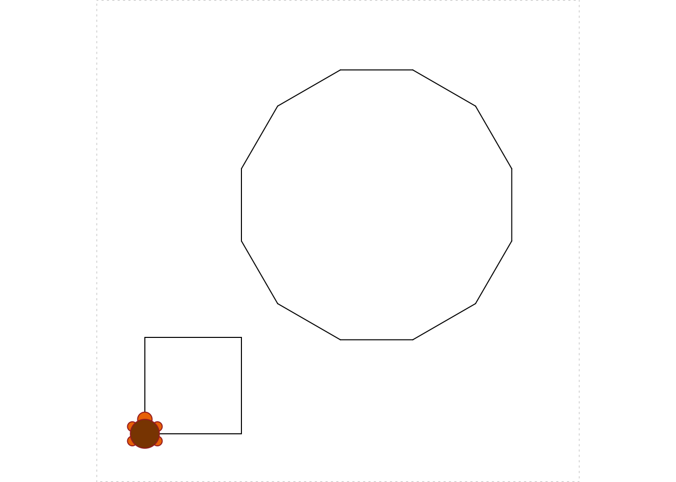
```
Figure 5.17: Testing the turtle_gon function

Note: You will use a loop when you write the function. It is important to wrap your loop in a call to turtle_do(), as in examples in this chapter, so the function will run quickly even when drawing polygons that have a lot of sides.
Write a function called turtle_star() that can make stars like the ones in Figure 5.18. Here are the required parameters:
- n: the number of rays in a star (default should be 6);
- length: the length of the rays (default should be 20);
- color: the color of the rays (default should be "red");
- type: the line-type of the rays (default should be 1);
- width: the line-width of the rays (default should be 1).
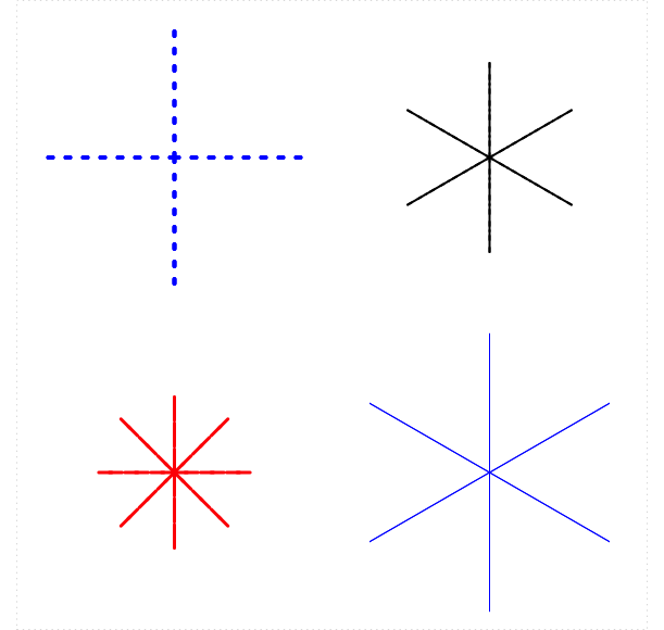
Figure 5.18: Sample Stars

Unlike the previous exercise, the body of your function should include the call turtle_init(mode = "clip"), so that a new field is created when the function is run and there is no error if the user asks for a star that extends outside the field.

Among the test for your function, include one that creates a star with 10 rays, each of length 20 units. The lines should be red and dashed. I’ll leave the thickness up to you.
Modify the function from the previous exerise to make a new star-function called turtle_rstar(), in which the lengths of the rays are not determined by the user but instead vary randomly from 5 to 25 units, as in Figure 5.19: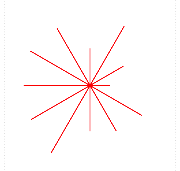

Figure 5.19: A star with rays of random lengths.

There is no longer a length parameter, but the names and default-values for the other parameters should be the same as in the previous exercise. Among the tests of the function, include one that makes a random star with 20 rays and a line-thickness of 3. (Other parameters should be left at their default-values.)

As in the previous exercise, please wrap your loop in a call to turtle_do().

Hint: You’ll use a loop to draw the rays of the star. As you go through the loop, get a random ray-length using the runif() function:
```
randomLength <- runif(1, min = 5, max = 25)
```
Then have the turtle make the ray by moving forward and backward by that amount.
Make a new star function turtle_rstarColors() that behaves like turtle_rstar() except that instead of being determined by the user the ray-color varies randomly from one ray to another, as in Figure 5.20: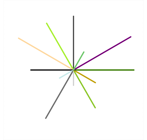

Figure 5.20: A star with rays of random lengths and random colors.

Each ray should have a color drawn randomly from the vector of all colors given by colors(). Among the tests of your function, include one that makes a random star with 20 rays and a line-thickness of 6. Other parameters should be left at their default-values.

Hint: You’ll use a loop to draw the rays of the star. As you go through the loop, get a new random color like this:
```
randomColor <- sample(colors(), size = 1)
```
Then set the turtle’s color accordingly:
```
turtle_col(col = randomColor)
```
(*) Our turtle_quick_pollack() function has successive strokes attached to each other. However, Jackson Pollack famous “drip” style involved placing brush-strokes at seemingly random locations on the canvas—successive strokes weren’t placed together. Modify our Pollack-painter function so that each new stroke appears as a random location inside the canvas. If you really get into it, research colors in R and try to come up with your own scheme for randomizing colors.

4 Flow-Control

6 Simulation