Exercises

Using the bcscr::m111survey data frame, write the ggplot2 code necessary to produce the graph in the figure below. (The points are all blue.)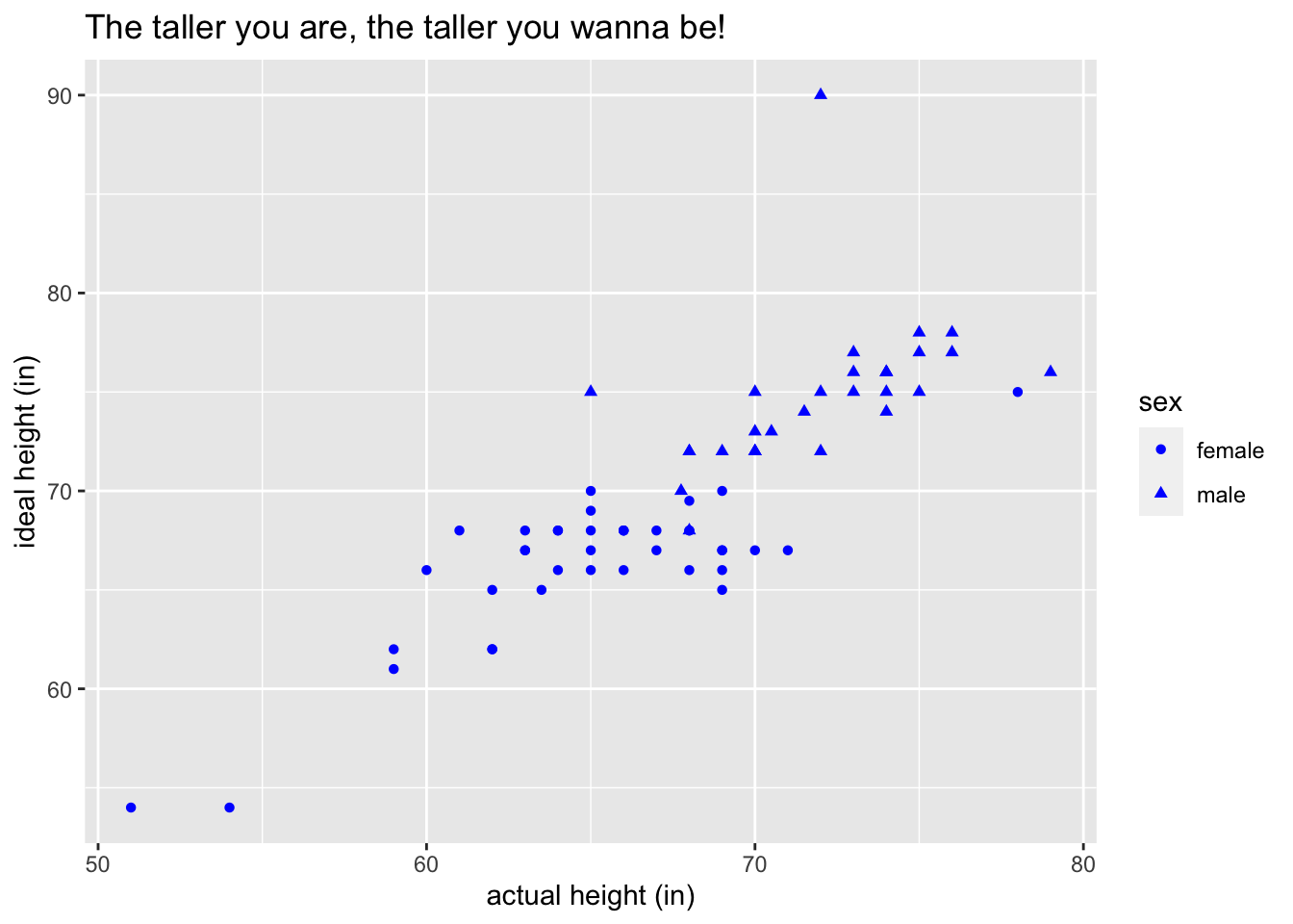

Hint: For the points, map the aesthetic property shape ot the variable sex. On the other hand, color is a fixed property.
Using the mosaicData::Utilities data frame, write the ggplot2 code necessary to produce the graph in the figure below.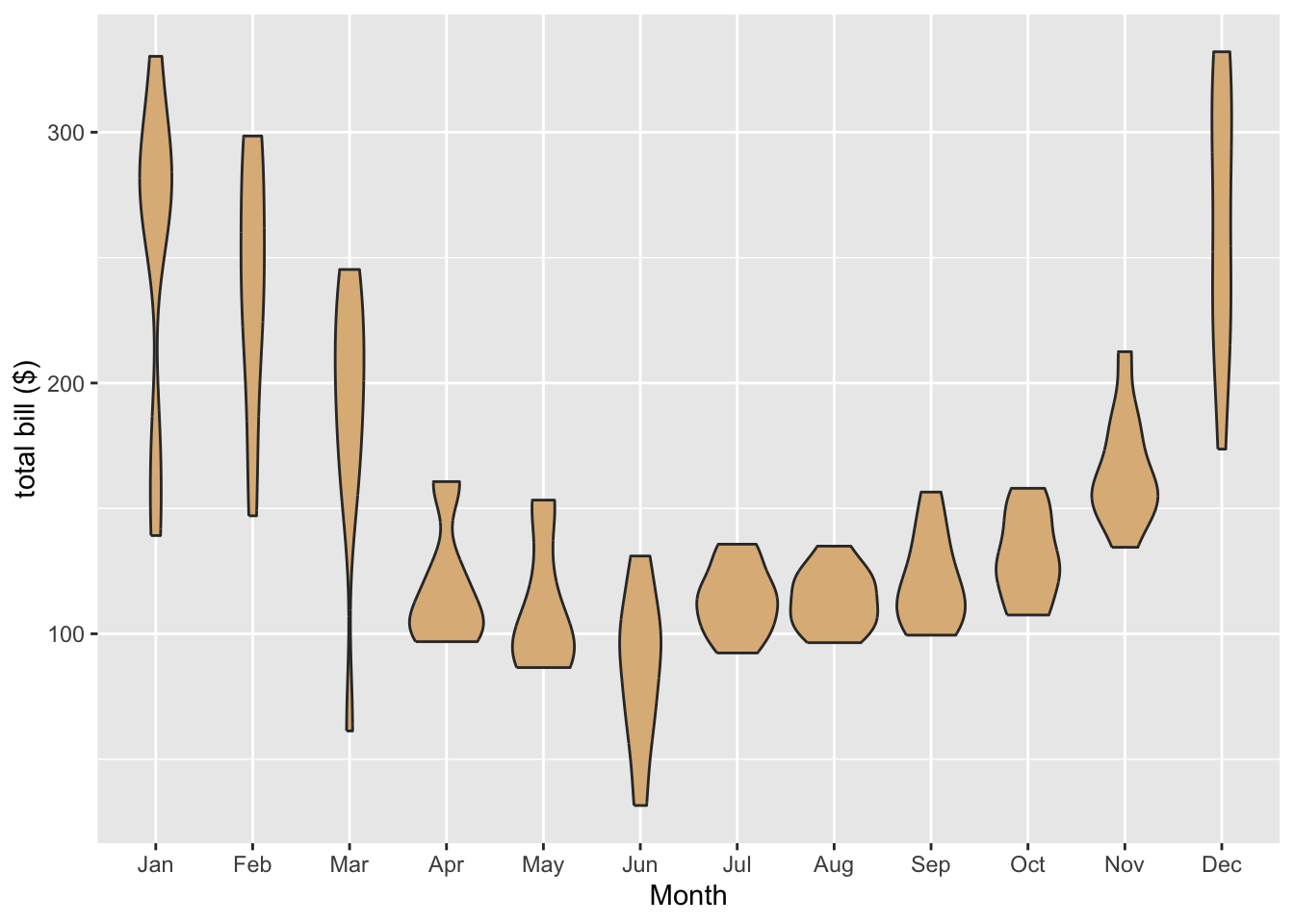

Hint: The month variable in Utilities is given numerically: 0 for January, 1 for February, and so on. You’ll need to use plyr::mapvalues() to map the numbers from 1 to 12 to the abbreviated month names. (See section 8.4 for a review of this.) The special R-vector month.abb will render the re-mapping task easy:
```
month.abb
```
```
##  [1] "Jan" "Feb" "Mar" "Apr" "May" "Jun" "Jul" "Aug" "Sep" "Oct" "Nov" "Dec"
```
In fact, you can create your new variable with abbreviated monnths with this code:
```
 monthAbbr <- with(Utilities, 
                  plyr::mapvalues(month, from = 1:12,
                                  to = month.abb))
```
You also need to make sure that the months come in the right order along the x-axis of the graph. To do this consider resetting the levels of your new monthAbbr variable. One way to accomplish this is to convert monthAbbr back to a factor with levels in the order you want, as done in Section 8.4, like this:
```
monthAbbr <- factor(monthAbbr, levels = month.abb)
```
Then you can put your new variable into the data frame, naming it anything you like:
```
Utilities$monthName <- monthAbbr
```
The next few exercises pertain to the data frame CPS85 from the package mosaicData. Learn about it with help(CPS85). We will use the ggplot2 graphing package to explore whether men were being paid more than women in 1985.

Make a density plot of the wages of the people in the study. As with all plots you make, it should have well-labelled axes (with units if possible). For a density plot you should label the horizontal axis, but you can let ggplo2 provide the label for the “density” axis. As always, provide a descriptive title. Also provide a “rug” of individual values along the horizontal axis.
Look at the plot you made in the previous exercise: you will notice that one person made a wage that was much higher than all the rest. In data analysis, when a value is much higher or lower than the rest of the values we call it an outlier.

Write the code needed to find the age, sex and sector of employment of the person who made this extraoridinarily high wage. Report the age, sex and sector of this person.

Create a new data frame called cpsSmall that is the same as CPS85 except that it excludes the row corresponding to the outlier-individual.
In order to explore the relationship between wage and sex in the CPS study, make violin plots for the wages of men and women. (In this exercise and in subsequent exercises, use the cpsSmall data frame so as to exclude the outlier.) Based on the plot, who tends to earn higher wages: men or women?
(*) Someone might argue that men don’t earn higher wages because of sex-discrimination in the workplace, but rather because of some other factor. For example, it could be that in 1985 women chose to work in low-wage sectors of the economy, whereas men tended to work in higher-wage sectors. Of course for this explanation to be viable, some sectors of the economy have to pay more on average than other sectors do. In order to verify whether this is the case, make a box plot of wage vs. sector of employment. Use the plot to name a couple of high-wage sectors and a couple of low-wage sectors.
(*) From the previous exercise you now know that some sectors of the economy pay more than other sectors. Hence in order to investigate properly whether there was wage-discrimination in the workforce based on sex, we would have to compare the wages of men and women who work in the same sector. To this end it would be nice to have eight separate box plots, one for each sector. Each plot would compare the wages of men and women in that sector. Use facet_wrap() to construct a graph that displays all eight plots at once.

Examine your graph.
- Are there any sectors in which it seems that women typically make more than men. If so, what sectors are they?
- On the other hand, are there any sectors where men typically make more than women? If so, what sectors are they?
- Based on your analysis, does it seem plausible that women made less than men simply because they chose lower-paying sectors of employment?