15.6 Application: Whales in an Ocean

Let’s now write a more elaborate program in the object-oriented style. Our program will simulate the population growth for whales in a ocean. In our model:

• Whales are mostly solitary: they move randomly about the ocean, happily feeding upon plankton.
• When a male and female whale are sufficiently close together the female whale will check out the male to see if he is mature enough to mate. If she herself is fertile, then she will mate with him and a child will be produced.
• That child will be either male or female, with equal likelihood for either option.
• After mating, the female will be infertile for a period of time.
• Whales have a set maximum lifetime.
• In any given time period, it is possible for a whale to starve, causing it to die before reaches its lifespan. The probability of starvation is low when the whale population is small (presumably there is plenty of plankton available then) but the starvation-probability increases in direct proportion to the population.

From the above conditions you can see that if the whale population is small then there is low probability of starvation, but on the other hand whales are liable to be spread thinly throughout the ocean. As a result males and females are relatively unlikely to run across each other, and hence births are less likely to occur. With a low enough population there is a strong possibility that the whales will die off before they can reproduce. (This is why biologists worry about some whale populations: if the whales are hunted to the point where the population is below a certain critical threshold, then they can go extinct on their own, even if hunting ceases.) On the other hand, if the whale population grows large then males and female meet frequently, and there are plenty of births. As the populations increases, however, food supplies dwindle, resulting in higher starvation rates. At some point birth and starvation balance each other out, resulting in a long-term equilibrium population-level.

We will implement our simulation with various objects:

• an ocean
• whales of two types:
  • male whales
  • female whales

We will begin by defining the class Whale:

Whale <- R6Class("Whale",
  public = list(
    position = NULL,
    age = NULL,
    lifespan = NULL,
    range = NULL,
    maturity = NULL,
    stepSize = NULL,
    initialize = function(position = NA, age = 3,
                          lifespan = 40, range = 5,
                          maturity = 10, stepSize = 5) {
      self$position <- position
      self$age <- age
      self$lifespan <- lifespan
      self$range <- range
      self$maturity <- maturity
      self$stepSize <- stepSize
    }
  )
)

For whales that are instances of the Whale class:

• position will contain the current x and y-coordinate of the whale in a two-dimensional ocean;
• age will give the current age of the whale.
• lifespan is the maximum age that the whale can attain before it dies.
• range is how close the whale has to be to another whale of the opposite sex in order to detect the presence of that whale.
• maturity is the age that the whale must attain in order to be eligible to mate.
• stepSize is the distance that the whale moves in the ocean in a single time-period.

Whales need to be able to move about in the sea. A whale moves by picking a random direction—any angle between 0 and \(2\pi\) radians—and then moving stepSize units in that direction. If the selected motion would take the whale outside the boundaries of the ocean, then R will repeat the motion until the whale lands properly within the boundaries.

The motion of a whale is implemented in the code below for a move() method that is added to class Whale:

Whale$set("public",
  "move",
  function(dims, r = self$stepSize) {
    xMax <- dims[1]
    yMax <- dims[2]
    repeat {
      theta <- runif(1, min = 0, max = 2 * pi)
      p <- self$position + r * c(cos(theta), sin(theta))
      within <- (p[1] > 0 && p[1] < xMax) && (p[2] > 0 && p[2] < yMax)
      if (within) {
        self$position <- p
        break
      }
    }
  },
  overwrite = TRUE
)

Note the parameter dims for the move function. From the code we can tell that it’s a vector of length 2. In fact the parameter will contain the x and and y-dimensions (the width and breadth) of our ocean. It’s something that will have to be determined by the ocean itself. We haven’t written the class Ocean yet, so this part of the code will have to remain a bit mysterious, for now.

We need male and female whales, so we create a class for each sex. Both classes inherit from Whale. The class Male adds only a sex attribute:

Male <- R6Class("Male",
  inherit = Whale,
  public = list(
    sex = "male"
  )
)

A female whale is a bit more complex: in addition to a sex attribute, she needs an attribute that specifies how long she will be infertile after giving birth, and another attribute that enables the program to keep track of the number of time-periods she must wait until she is fertile again:

Female <- R6Class("Female",
  inherit = Whale,
  public = list(
    sex = "female",
    timeToFertility = 0,
    infertilityPeriod = 5
  )
)

A female whale also needs a method to determine whether a mature whale is in the vicinity:

Female$set("public",
  "maleNear",
  function(males, dist) {
    foundOne <- FALSE
    for (male in males) {
      near <- dist(male$position, self$position) < self$range
      mature <- (male$age >= male$maturity)
      if (near && mature) {
        foundOne <- TRUE
        break
      }
    }
    foundOne
  },
  overwrite = TRUE
)

Again, note the parameters males and dist. Values for these parameters will be provided by the ocean object. males will be a list of the male whales in the population at the current time, and dist will be a function for computing the distance between any two points in the ocean.

A female whale also needs to be able to mate:

Female$set("public",
  "mate",
  function() {
    babySex <- sample(c("female", "male"), size = 1)
    self$timeToFertility <- self$infertilityPeriod
    return(babySex)
  },
  overwrite = TRUE
)

Now it is time to define the Ocean class. It’s a bit of a mouthful:

Ocean <- R6Class("Ocean",
  public = list(
    dimensions = NULL,
    males = NULL,
    females = NULL,
    malePop = NULL,
    femalePop = NULL,
    starveParameter = NULL,
    distance = function(a, b) {
      sqrt((a[1] - b[1])^2 + (a[2] - b[2])^2)
    },
    initialize = function(dims = c(100, 100),
                          males = 10,
                          females = 10,
                          starve = 5) {
      self$dimensions <- dims
      xMax <- dims[1]
      yMax <- dims[2]
      maleWhales <- replicate(
        males,
        Male$new(
          age = 10,
          position = c(
            runif(1, 0, xMax),
            runif(1, 0, yMax)
          )
        )
      )
      femaleWhales <- replicate(
        females,
        Female$new(
          age = 10,
          position = c(
            runif(1, 0, xMax),
            runif(1, 0, yMax)
          )
        )
      )
      self$males <- maleWhales
      self$females <- femaleWhales
      self$malePop <- males
      self$femalePop <- females
      self$starveParameter <- starve
    },
    starvationProbability = function(popDensity) {
      self$starveParameter * popDensity
    }
  )
)

In an instantiation of the class Ocean:

• dimensions will be numerical vector of length 2 that specifies the width and breadth of the ocean.
• males and females will be lists that contain respectively the current sets of male whales and female whales. Note that this implies that an ocean will contain as members other items that are themselves R6 classes. This is an example of what is called composition in object-oriented programming.
• malePop and femalePop give respectively the current counts male and females whales.
• starveParameter helps determine the probability that each individual whale will starve within the next time-period. Note that the method starvationProbability() makes the probability of starvation equal product of starveParameter and the current density of the population of whales in the ocean. The bigger this attribute is, the more starvation will occur and the lower the long-term upper limit of the population will be.
• distance() is the method for finding the distance between any two positions in the ocean. It implements the standard distance-formula from high-school geometry.
• The initialization function permits the user to determine the dimensions of the ocean, the initial number of male and female whales, and the starvation parameter. In the instantiation process for an individual ocean the required number of male and female whales are instantiated and are placed randomly in the ocean.

We need to add a method that allows an ocean to advance one unit of time. During that time:

• Each mature and fertile female whale must check for nearby mature males, mate with one if possible, and produce a baby.
• Any offspring produced must then be added to the ocean’s lists of male and female whales.
• The ocean must then subject each whale to the possibility of starvation within the time-period at hand.
• All whales that survive must then move.
• The age of each whale must be increased by one time-unit. For females, the time remaining until fertility must also be decreased by a unit.

The advance() method is implemented and added to Ocean with the code below:

Ocean$set("public",
  "advance",
  function() {
    malePop <- self$malePop
    femalePop <- self$femalePop
    population <- malePop + femalePop
    if (population == 0) {
      return(NULL)
    }
    males <- self$males
    females <- self$females
    babyMales <- list()
    babyFemales <- list()
    if (malePop > 0 && femalePop > 0) {
      for (female in females) {
        if (female$age >= female$maturity &&
          female$timeToFertility <= 0 &&
          female$maleNear(
            males = males,
            dist = self$distance
          )) {
          outcome <- female$mate()
          if (outcome == "male") {
            baby <- Male$new(age = 0, position = female$position)
            babyMales <- c(babyMales, baby)
          } else {
            baby <- Female$new(age = 0, position = female$position)
            babyFemales <- c(babyFemales, baby)
          }
        }
      }
    }

    # augment the male and female lists if needed:
    lmb <- length(babyMales)
    lfb <- length(babyFemales)

    # throw in the babies:
    if (lmb > 0) {
      males <- c(males, babyMales)
    }
    if (lfb > 0) {
      females <- c(females, babyFemales)
    }

    # revise population for new births:
    population <- length(males) + length(females)

    # starve some of them, maybe:
    popDen <- population / prod(self$dimensions)
    starveProb <- self$starvationProbability(popDensity = popDen)
    maleDead <- logical(length(males))
    femaleDead <- logical(length(females))
    # starve some males
    for (i in seq_along(maleDead)) {
      male <- males[[i]]
      maleDead[i] <- (runif(1) <= starveProb)
      male$age <- male$age + 1
      if (male$age >= male$lifespan) maleDead[i] <- TRUE
      if (maleDead[i]) next
      # if whale is not dead, he should move:
      male$move(dims = self$dimensions)
    }
    # starve some females
    for (i in seq_along(femaleDead)) {
      female <- females[[i]]
      femaleDead[i] <- (runif(1) <= starveProb)
      female$age <- female$age + 1
      if (female$age >= female$lifespan) femaleDead[i] <- TRUE
      if (femaleDead[i]) next
      if (female$sex == "female") {
        female$timeToFertility <- female$timeToFertility - 1
      }
      # if female is not dead, she should move:
      female$move(dims = self$dimensions)
    }

    # revise male and female whale lists:
    malePop <- sum(!maleDead)
    self$malePop <- malePop
    femalePop <- sum(!femaleDead)
    self$femalePop <- femalePop
    if (malePop > 0) {
      self$males <- males[!maleDead]
    } else {
      self$males <- list()
    }
    if (femalePop > 0) {
      self$females <- females[!femaleDead]
    } else {
      self$females <- list()
    }
  },
  overwrite = TRUE
)

In simulations we might enjoy looking at a picture of the ocean at any given time moment. Hence we add a plot() method that enables an ocean to produce a graph of the whales within it. In this graph males will be colored red and females green. Mature whales will appear as larger than immature whales. For purposes of speed we use R’s base graphics system rather than ggplot2.

Ocean$set("public",
  "plot",
  function() {
    males <- self$males
    females <- self$females
    whales <- c(males, females)
    if (length(whales) == 0) {
      plot(0, 0, type = "n", main = "All Gone!")
      box(lwd = 2)
      return(NULL)
    }
    df <- purrr::map_dfr(whales, function(x) {
      list(
        x = x$position[1],
        y = x$position[2],
        sex = as.numeric(x$sex == "male"),
        mature = as.numeric(x$age >= x$maturity)
      )
    })
    # males will be red, females green:
    df$color <- ifelse(df$sex == 1, "red", "green")
    # mature whales have cex = 3, immature whales cex 0.7
    df$size <- ifelse(df$mature == 1, 1.3, 0.7)
    with(
      df,
      plot(x, y,
        xlim = c(0, self$dimensions[1]),
        ylim = c(0, self$dimensions[1]), pch = 19, xlab = "",
        ylab = "", axes = FALSE, col = color, cex = size,
        main = paste0("Population = ", nrow(df))
      )
    )
    box(lwd = 2)
  },
  overwrite = TRUE
)

Finally, we write a simulation function. The function allows the user to specify the number of time-units that the simulation will cover, along with initial numbers of male and female whales. The user will have an option to “animate” the simulation showing a plot of the ocean after each time-unit. If the animation option is chosen, then R will use the Sys.sleep() function to make the computer suspend computations for half a second so that the user can view the plot. The simulation will cease if all of the whales die prior to end of the allotted time. Finally, the function uses ggplot2 to produce a graph of the whale population as a function of time.

library(ggplot2)
oceanSim <- function(steps = 100, males = 10, females = 10,
                     starve = 5, animate = TRUE, seed = NULL) {
  if (!is.null(seed)) {
    set.seed(seed)
  }
  ocean <- Ocean$new(
    dims = c(100, 100), males = males,
    females = females, starve = starve
  )
  population <- numeric(steps)
  for (i in 1:steps) {
    population[i] <- ocean$malePop + ocean$femalePop
    if (animate) ocean$plot()
    if (population[i] == 0) break
    ocean$advance()
    if (animate) Sys.sleep(0.5)
  }
  pop <- population[1:i]
  df <- data.frame(
    time = 1:length(pop),
    pop
  )
  ggplot(df, aes(x = time, y = pop)) + geom_line() +
    labs(x = "Time", y = "Whale Population")
}

We are now ready for a simulation. The results are graphed in Figure 15.1.

oceanSim(
  steps = 200, males = 15, females = 15,
  animate = FALSE, seed = 3030
)

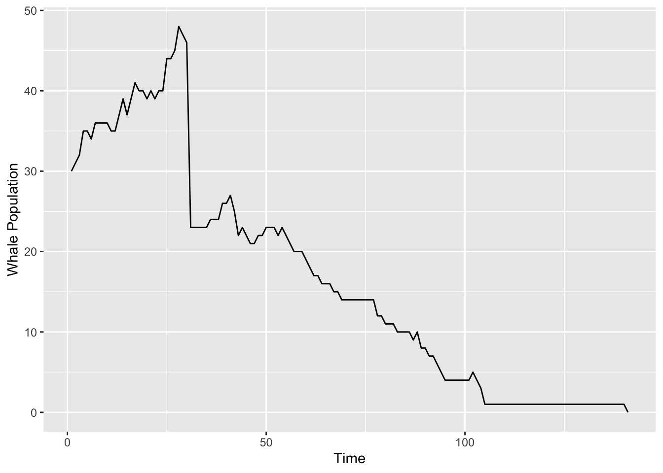
Figure 15.1: Simulated whale population. Sadly, they all die after about 130 days.

You should try running the simulation yourself a few times, for differing initial numbers of whales. If you like you can watch the whales move about by setting animate to TRUE:

oceanSim(
  steps = 200, males = 15, females = 15,
  animate = TRUE
)

You might also wish to explore varying the starve parameter: recall that the higher it is, the lower the long-term stable whale population will be. In order to better detect long-term stable population sizes, you will want to work with more steps, and you should turn off the step-by-step-animation, thus:

oceanSim(
  steps = 1000, males = 75, females = 75,
  starve = 2.5, animate = FALSE
)

The R package bcscr ((White 2021)) includes a more flexible version of the Ocean class that allows the users to set custom initial populations, including characteristics that vary from whale to whale.

The object-oriented approach to simulation is not necessarily the quickest approach: R6 objects do require a bit more time for computation, as compared to a system that stores relevant information about the population in vectors or in a data frame. On the other hand the object-oriented approach makes it easy to encode information about each individual whale as it proceeds through time. In larger applications, an object-oriented approach to programming can result in code that is relatively easy to read and to modify, albeit at some cost in terms of speed.