6.8 Example: The Drunken Turtle
Let us return to the scenario of the Drunken Turtle that was introduced in Section 5.4.5. At each step the turtle would turn by a random angle—any angle between 0 and 360 degrees with equal likelihood—and then move forward by a fixed number of units. We wondered whether the turtle would simply wander away from its starting point or perhaps eventually loop back close to its starting point.
In this section we will construct a simulation that sheds light on our question. We will imagine that the turtle starts at the origin on the \(xy\)-plane and takes a large but fixed number of steps—one thousand steps, say—each of a fixed length of one unit, but each of which is preceded by a drunken turn through a random angle. We will concern ourselves with the random variable \(X\), defined as follows:
\(X\) = the number of times in the turtle returns to within \(1/2\) of a unit of the origin, during its first 1000 steps.
(Apparently we consider a “close return” to be anything within half a unit of the origin.)
In particular, we would like to know the distribution of \(X\): what is the chance that the turtle does not make a close return during the first thousand steps? What’s the chance of making only one close return? Two close returns? And so on … . We would also like to estimate the expected value of \(X\): the average number of close returns in the first 1000 steps.
We will next consider how to code a simulation. Obviously we will need a way to record the turtle’s position at each step. In order to accomplish this we will have to apply the unit-circle trigonometry you learned in high school.
Instead of measuring angles in degrees, we will work in radians: by default R does trigonometry that way. Recall that 360 degrees is \(2 \pi\) radians; hence the way to determine the angle of a turn by the drunken turtle is with the following call to runif():
runif(1, min = 0, max = 2*pi)## [1] 4.146176If we want a thousand drunken turn-angles, then we can get them all in a vector, as follows:
runif(1000, min = 0, max = 2*pi)So much for the turning angles. But in order to decide at each step whether the turtle has made a close return, we have to know the coordinates of the turtle after each step. This is where unit-circle trigonometry comes in handy. Recall that if a right triangle has a hypotenuse of length 1 (the length of a turtle step) and if one of the angles of the triangle is \(\alpha\), then the side adjacent to \(\alpha\) is \(\cos(\alpha)\) and the side opposite is \(\sin(\alpha)\). The situation is illustrated in Figure 6.4.
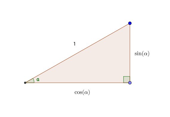
Figure 6.4: Sides of a right triangle with hypotenuse 1, in terms of the angle shown.
From this principle it follows that if the turtle turns a random angle of \(a_1\) radians for its first step, then after it takes the one-unit step it will be at the point \((\cos(a_1), \sin(a_2))\).
For the second step, the turtle begins by turning another random angle, say \(a_2\) radians. It then takes another one-unit step. This second step forms the hypotenuse of a second right triangle (see Figure 6.5). The horizontal and vertical sides of this right triangle must be \(\cos(a_2)\) and \(\sin(a_2)\) respectively. When the turtle complete the second step, it has added these values to its previous \(x\) and \(y\) coordinates, so that it is now at the point:
\[(\cos(a_1) + \cos(a_2), \sin(a_1) +\sin(a_2)).\] We now see the idea: in order to record the position of the turtle at the end of each step, we simply need to:
- take the cosine of all the turning-angles;
- take the sine of all the turning-angles;
- sum the cosines to get the \(x\)-coordinate;
- sum the sines to get the \(y\)-coordinate.
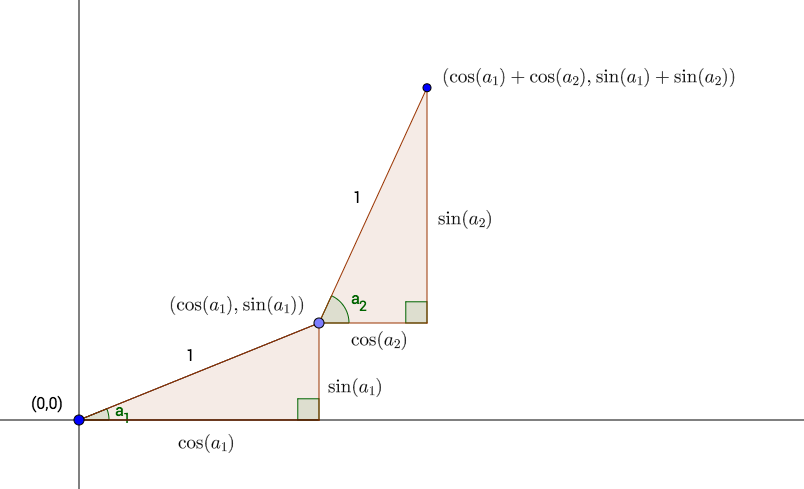
Figure 6.5: The first two steps by the Drunken Turtle. Turtle turns by \(a_1\) radians for Step One, then by \(a_2\) radians for Step Two.
Let’s put this idea into practice, for just the first ten steps. First, get the turning angles, the sines and the cosines:
angle <- runif(10, 0 , 2*pi)
xSteps <- cos(angle)
ySteps <- sin(angle)
Next, we need to add the xSteps together. If we do a sum, we would get the \(x\)-coordinate after the tenth step:
sum(xSteps)## [1] -1.370258(Apparently some of the cosines were negative, meaning that some of the turning angles were between 90 and 270 degrees.)
We need the \(x\)-coordinates after all of the previous steps, as well. This can be accomplished by R’s cumsum() function. You may think of cumsum as short for “cumulative sum.” Given a vector vec of numbers, cumsum(vec) returns a vector of the same length, where for every index i, cumsum(vec)[i] is sum(vec[1:i]). This is made clear in the following example:
vec <- c(3, 2, -1, 4, -2)
cumsum(vec)
## [1] 3 5 4 8 6Look at the table below.
vec |
cumulative sum | cumsum(vec) |
|---|---|---|
| 3 | 3 | 3 |
| 2 | \(3+2\) | 5 |
| -1 | \(3+2+-1\) | 4 |
| 4 | \(3+2+-1+4\) | 8 |
| -2 | \(3+2+-1+4+-2\) | 6 |
See how it works?
Returning to xSteps, we see that we can get the \(x\)-coordinates of the first ten steps like this:
x <- cumsum(xSteps)
x
## [1] -0.6034165 -1.3905805 -2.1259607 -3.1154380 -2.4593130 -1.5476110 -0.8591924
## [8] -1.6420445 -0.6421761 -1.3702583Similarly we can get the first ten \(y\)-coordinates:
y <- cumsum(ySteps)Using the distance formula, we can compute the distance of each point from the origin as follows:
dist <- sqrt(x^2 + y^2)The following logical vector will then record, at each each step, whether or not the turtle has made a close return:
closeReturn <- (dist < 0.5)The results are shown in Table 6.3.
| angle | xSteps | ySteps | x | y | dist | closeReturn |
|---|---|---|---|---|---|---|
| 4.0646104 | -0.6034165 | -0.7974262 | -0.6034165 | -0.7974262 | 1.000000 | FALSE |
| 2.4769935 | -0.7871641 | 0.6167437 | -1.3905805 | -0.1806826 | 1.402270 | FALSE |
| 3.8861615 | -0.7353801 | -0.6776548 | -2.1259607 | -0.8583374 | 2.292695 | FALSE |
| 2.9963954 | -0.9894774 | 0.1446876 | -3.1154380 | -0.7136497 | 3.196131 | FALSE |
| 0.8551238 | 0.6561251 | 0.7546522 | -2.4593130 | 0.0410024 | 2.459655 | FALSE |
| 0.4233886 | 0.9117020 | 0.4108522 | -1.5476110 | 0.4518546 | 1.612226 | FALSE |
| 0.8114898 | 0.6884186 | 0.7253136 | -0.8591924 | 1.1771682 | 1.457373 | FALSE |
| 2.4700328 | -0.7828521 | 0.6222079 | -1.6420445 | 1.7993761 | 2.435993 | FALSE |
| 0.0162276 | 0.9998683 | 0.0162269 | -0.6421761 | 1.8156030 | 1.925826 | FALSE |
| 3.8968689 | -0.7280822 | -0.6854899 | -1.3702583 | 1.1301131 | 1.776165 | FALSE |
It remains only to package our code into a simulation function. We will allow the user to specify the fixed initial number of steps (it does not have to be 1000), and also to determine what distance counts as a “close return.”
drunkenSim <- function(steps = 1000, reps = 10000, close = 0.5,
                       seed = NULL, table = FALSE) {
  if ( !is.null(seed) ) {
    set.seed(seed)
  }

  # set up returns vector to store the number of
  # close returns in each repetition:
  returns <- numeric(reps)

  for (i in 1:reps) {
  angle <- runif(steps, 0 , 2*pi)
  xSteps <- cos(angle)
  ySteps <- sin(angle)

  x <- cumsum(xSteps)
  y <- cumsum(ySteps)

  dist <- sqrt(x^2 + y^2)
  closeReturn <- (dist < 0.5)
  returns[i] <- sum(closeReturn)
  }

  if ( table ) {
    cat("Here is a table of the number of close returns:\n\n")
    tab <- prop.table(table(returns))
    print(tab)
    cat("\n")
  }
  cat("The average number of close returns was:  ",
      mean(returns), ".", sep = "")
}
Let’s try it out:
drunkenSim(steps = 1000, reps = 10000,
           close = 0.5, seed = 3535, table = TRUE)
## Here is a table of the number of close returns:
##
## returns
## 0 1 2 3 4 5 6 7 8 9 10 11
## 0.3881 0.2290 0.1517 0.0908 0.0572 0.0335 0.0227 0.0107 0.0064 0.0048 0.0018 0.0012
## 12 13 14 15 16 17
## 0.0008 0.0007 0.0003 0.0001 0.0001 0.0001
##
## The average number of close returns was: 1.5655.Notice that 38.81% of the time the turtle did not make a close return at all during the first thousand steps. On the other hand it is possible, though not at all likely, for the turtle to make quite a few close returns.22
It is interesting to look specifically at the distances from the origin. The following function draws a graph of the distance from the origin for the specified number of turtle steps:
drunkenSim2 <- function(steps = 1000, seed = NULL) {
  if ( !is.null(seed) ) {
    set.seed(seed)
  }

  angle <- runif(steps, 0 , 2*pi)
  xSteps <- cos(angle)
  ySteps <- sin(angle)
  x <- cumsum(xSteps)
  y <- cumsum(ySteps)
  dist <- sqrt(x^2 + y^2)
  plotTitle <- paste0("First ", steps, " Steps of the Drunken Turtle")
  p <- ggplot(mapping = aes(x = 1:steps, y=dist)) + geom_line() +
    labs(x = "Step", y = "Distance From Origin",
         title = plotTitle)
  print(p)
}
Let’s try it out! The results appear in Figure 6.6
drunkenSim2(steps = 1000, seed = 2525)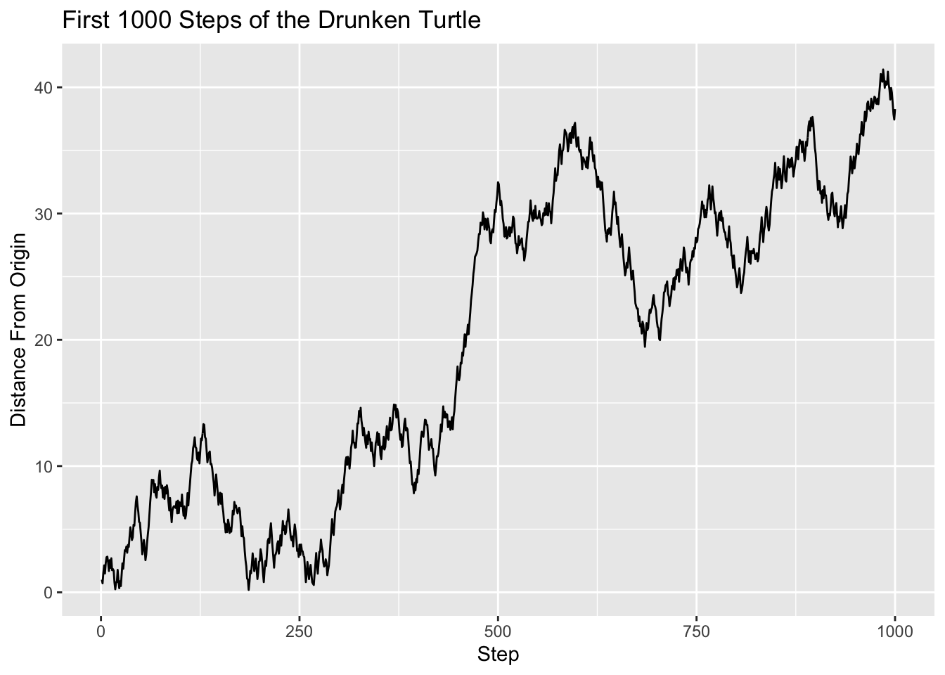
Figure 6.6: Line plot of the Turtle’s distance from the origin, as a function of how many steps the turtle has taken.
It appears that although the turtle might have returned close to the origin a couple of times, for the most part it seems to be wandering further and further away. In the mathematical field known as stochastic processes, it has been shown that if the turtle is allowed to go on forever then it will certainly make a close return infinitely many times. These returns, though, will tend to be spaced further and further apart as time goes on, and our graph suggests that this is so.
Note that these proportions depend heavily on how we define “close.” If the cut-off had been lower than \(1/2\), then we would have seen fewer close returns.↩︎