10 Basic Tidyverse Concepts

Figure 10.1: The Treachery of Images (Rene Magritte, 1948).

In this chapter we will introduce a few tools from the tidyverse set of R-packages:

the pipe operator %>% for chaining function calls in a convenient and readable way;
the tibble class, a variant of the data frame that is especially suitable for large data sets;
data manipulation functions from the dplyr package suitable for use with the pipe operator:
- filter() and select() for sub-setting;
- mutate() for transforming variables;
- group_by() and summarise() for numerical summaries of data.

10.1 The Tidyverse

The tidyverse isn’t a package, exactly—it’s a collection of packages. Go ahead and attach it:

library(tidyverse)

You’ll get an account of the packages that have been attached. We have worked before with ggplot and by the end of CSC 215 we will have worked with all of the others. You need not worry about the fact that filter() and lag() mask functions from the stats package.

10.2 The magrittr Pipe Operator

In Section 6.8.4 you met R’s native pipe operator |>. The tidyverse uses another pipe operator, %>% from the magrittr package.²⁶.

The keyboard shortcut for %>% is:

Ctrl+Shift+M on Windows/Linux, or
Cmd+Shift+M on Mac OS.

The the native R pipe operator, %>% connects two function calls by making the value returned by the first call the first argument of the second call. Here’s an example:

"hello" %>% rep(times = 4)

## [1] "hello" "hello" "hello" "hello"

This is the same as the more familiar:

rep("hello", times = 4)

## [1] "hello" "hello" "hello" "hello"

Here’s another example:

# same as nrow(bcscr::m111survey)
bcscr::m111survey %>% nrow()

## [1] 71

Here’s two pipes:

"hello" %>% rep(times = 4) %>% length()

## [1] 4

By default the value of the left-hand call is piped into the right-hand call as the first argument. You can make it some other argument using the dot . as a placeholder, for example:

4 %>% rep("hello", times = .)

## [1] "hello" "hello" "hello" "hello"

(Recall that the placeholder for the native R pipe is _. Do not interchange _ with .)

Since sub-setting is actually a function call under the hood, you can use the dot there, too:

# gets the third element of the sequence 1, 4, 9, ..., 97:
seq(1, 100, by = 4) %>% .[3]

## [1] 9

The pipe operator isn’t all that useful when you only use it once or twice in succession. Its true value becomes apparent in the chaining together of many manipulations involving data frames.

10.2.1 Practice Exercises

Rewrite the following call with the tidyverse pipe operator, in three different ways:
```
seq(2, 22, by = 4)
```
```
## [1]  2  6 10 14 18 22
```
Consider mosaicData::CPS85:
```
data("CPS85", package = "mosaicData")
```
Use the pipe operator with subset() to find the row of mosaicData::CPS85 containing the worker who made more than 40 dollars per hour. Display only the sex, age and wage of the worker.

10.2.2 Solutions to the Practice Exercises

Here are three ways:

2 %>% seq(22, by = 4)
22 %>% seq(2, ., by = 4)
4 %>% seq(2, 22, by = .)

Try this:

CPS85 %>% 
  subset(wage > 40) %>% 
  .[, c("sex", "age", "wage")]

##     sex age wage
## 249   F  21 44.5

10.3 Tibbles

The tibble package gives us tibbles, which are very nearly the same thing as a data frame. Indeed, the name “tibble” is supposed to remind us of a data “table.”

Consider the class of bcscr::m111survey:

class(bcscr::m111survey)

## [1] "data.frame"

Yep, it’s a data frame. But we can convert it to a tibble, as follows:

survey <- as_tibble(bcscr::m111survey)
class(survey)

## [1] "tbl_df"     "tbl"        "data.frame"

You can treat tibbles like data frames. For now the primary practical difference is manifest when you print a tibble to the Console:

survey

## # A tibble: 71 × 12
##    height ideal_ht sleep fastest weight_feel   love_first extra_life
##     <dbl>    <dbl> <dbl>   <int> <fct>         <fct>      <fct>     
##  1   76         78   9.5     119 1_underweight no         yes       
##  2   74         76   7       110 2_about_right no         yes       
##  3   64         NA   9        85 2_about_right no         no        
##  4   62         65   7       100 1_underweight no         no        
##  5   72         72   8        95 1_underweight no         yes       
##  6   70.8       NA  10       100 3_overweight  no         no        
##  7   70         72   4        85 2_about_right no         yes       
##  8   79         76   6       160 2_about_right no         yes       
##  9   59         61   7        90 2_about_right no         yes       
## 10   67         67   7        90 3_overweight  no         no        
## # ℹ 61 more rows
## # ℹ 5 more variables: seat <fct>, GPA <dbl>, enough_Sleep <fct>,
## #   sex <fct>, diff.ideal.act. <dbl>

The output is automatically truncated, and the number of columns printed is determined by the width of your screen. This is a great convenience when one is dealing with larger data sets.

Many larger data tables in packages will come to you as tibbles.

10.4 Subsetting with dplyr

The dplyr function filter() is the rough equivalent of select(): it picks out rows of a data frame (or similar objects such as a tibble). The dplyr function select() subsets for columns.

Thus you can use the two functions together to do perform sub-setting. With the pipe operator, your code can be quite easy to read:

survey %>% 
  filter((sex == "male" & height > 70) | (sex =="female" & height < 55)) %>% 
  select(sex, height, fastest)

## # A tibble: 22 × 3
##    sex    height fastest
##    <fct>   <dbl>   <int>
##  1 male     76       119
##  2 male     74       110
##  3 male     72        95
##  4 male     70.8     100
##  5 male     79       160
##  6 male     73       110
##  7 male     73       120
##  8 female   54       130
##  9 male     74       119
## 10 male     72       125
## # ℹ 12 more rows

Note that dplyr data-functions like filter() and select() take a data table as their first argument, and return a data table as well. Hence they may be chained together as we saw in the above example.

With select() it’s easy to leave out columns, too:

survey %>% 
  select(-ideal_ht, -love_first)

## # A tibble: 71 × 10
##    height sleep fastest weight_feel   extra_life seat       GPA
##     <dbl> <dbl>   <int> <fct>         <fct>      <fct>    <dbl>
##  1   76     9.5     119 1_underweight yes        1_front   3.56
##  2   74     7       110 2_about_right yes        2_middle  2.5 
##  3   64     9        85 2_about_right no         2_middle  3.8 
##  4   62     7       100 1_underweight no         1_front   3.5 
##  5   72     8        95 1_underweight yes        3_back    3.2 
##  6   70.8  10       100 3_overweight  no         1_front   3.1 
##  7   70     4        85 2_about_right yes        1_front   3.68
##  8   79     6       160 2_about_right yes        3_back    2.7 
##  9   59     7        90 2_about_right yes        3_back    2.8 
## 10   67     7        90 3_overweight  no         2_middle NA   
## # ℹ 61 more rows
## # ℹ 3 more variables: enough_Sleep <fct>, sex <fct>,
## #   diff.ideal.act. <dbl>

10.4.1 Practice Exercises

Can you use the pipe to chain dplyr functions along with nrow() to find out how many people in survey believe in love at first sight and drove more than 120 miles per hour?
Find the three largest heights of the males who drove more than 120 miles per hour.
Use the pipe and filter() to make violin plots of the wages of men and women in CPS85, where the outlier-person (whose wage was more than 40 dollars per hour) has been eliminated prior to making the graph.

10.4.2 Solutions to Practice Exercises

Try this:

survey %>% 
  filter(love_first == "yes" & fastest > 120) %>% 
  nrow()

## [1] 3

Here’s one way:

survey %>% 
  filter(sex == "male" & fastest > 120) %>%
  .$height %>%                 # this is just a vector
  sort(decreasing = TRUE) %>%  # so you can sort it ... 
  .[1:3]                       # then get its first three elements

## [1] 79 75 75

Try this code:

CPS85 %>% 
  filter(wage <= 40) %>% 
  ggplot(aes(x = sex, y = wage)) +
    geom_violin(fill = "burlywood")

10.5 Transforming Variables with dplyr

In dplyr you transform variables with the function mutate(). Here is an example:

survey %>% 
  mutate(dareDevil = fastest > 125) %>%
  select(sex, fastest, dareDevil)

## # A tibble: 71 × 3
##    sex    fastest dareDevil
##    <fct>    <int> <lgl>    
##  1 male       119 FALSE    
##  2 male       110 FALSE    
##  3 female      85 FALSE    
##  4 female     100 FALSE    
##  5 male        95 FALSE    
##  6 male       100 FALSE    
##  7 male        85 FALSE    
##  8 male       160 TRUE     
##  9 female      90 FALSE    
## 10 female      90 FALSE    
## # ℹ 61 more rows

In mutate() there is always a variable-name on the left-hand side of the = sign. It could be the same as an existing variable in the table if you are content to overwrite that variable. On the right side of the = is a function that can depend on variables in the data table.

You can transform more than one variable in a single call to mutate(), as in the code below. The output is shown in 10.2.

survey %>% 
  mutate(dareDevil = fastest > 125,
         height_ft = height / 12) %>% 
  ggplot(aes(x = dareDevil, y = height_ft)) +
    geom_boxplot(fill = "burlywood", out.alpha = 0) +
    geom_jitter(width = 0.2) +
  labs(
    x = "Whether person drives more than 125 mph",
    y = "height (ft)",
    title = "Daredevils aren't any taller than cautious people!"
  )

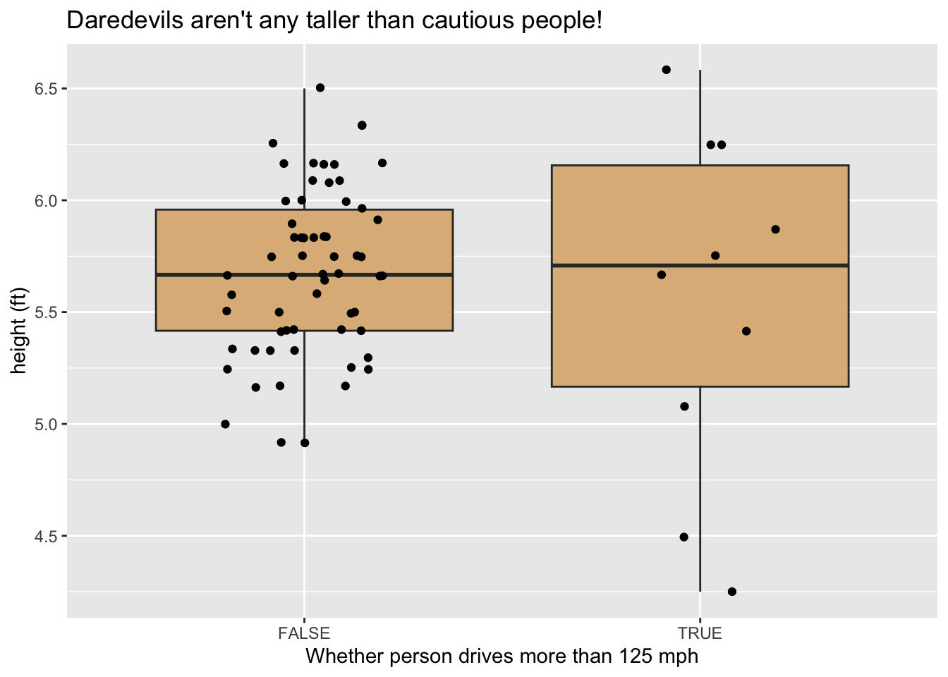
Figure 10.2: Graph produced after mutation.

10.5.1 Practice Exercises

In mosaicData::CPS85 transform the wage variable to units of dollars per day. (Assume an 8-hour working day.)

10.5.2 Solutions to Practice Exercises

Try this:

CPS85 %>% 
  as_tibble() %>%                   # for display in Console
  mutate(dailyWage = wage * 8) %>% 
  select(sex, sector, dailyWage)    # for display in Console

## # A tibble: 534 × 3
##    sex   sector   dailyWage
##    <fct> <fct>        <dbl>
##  1 M     const         72  
##  2 M     sales         44  
##  3 F     sales         30.4
##  4 F     clerical      84  
##  5 M     const        120  
##  6 F     clerical      72  
##  7 F     service       76.6
##  8 M     sales        120  
##  9 M     manuf         88  
## 10 F     sales         40  
## # ℹ 524 more rows

10.6 Grouping and Summaries

The next two dplyr data-functions are useful for generating numerical summaries of data.

Consider, for example, CPS85. We know from graphical studies that the men in the study are paid more than women, but how might we verify this fact numerically? One approach would be to separate the men and the women into two different groups and compute the mean wage for each group. This is accomplished by calling group_by() and summarise() in succession:

CPS85 %>% 
  group_by(sex) %>% 
  summarize(meanWage = mean(wage))

## # A tibble: 2 × 2
##   sex   meanWage
##   <fct>    <dbl>
## 1 F         7.88
## 2 M         9.99

It’s possible to create more than one summary variable in a single call to summarise(), for example:

CPS85 %>% 
  group_by(sex) %>% 
  summarize(
    meanWage = mean(wage),
    n = n()
  )

## # A tibble: 2 × 3
##   sex   meanWage     n
##   <fct>    <dbl> <int>
## 1 F         7.88   245
## 2 M         9.99   289

In the previous example, dplyr::n() was used to count the number of cases in each group.

For a more complete account of a numerical variable, one might consider the five-number summary:

the minimum value
the first quartile (Q1)
the median
the third quartile (Q3)
the maximum value

These quantities are conveniently computed by R’s fivenum() function:

CPS85 %>% 
  .$wage %>% 
  fivenum()

## [1]  1.00  5.25  7.78 11.25 44.50

Let’s find the five number summaries for the wages of men and women:

CPS85 %>%
  group_by(sex) %>% 
  summarise(
    n = n(),
    min = fivenum(wage)[1],
    Q1 = fivenum(wage)[2],
    median = fivenum(wage)[3],
    Q3 = fivenum(wage)[4],
    max = fivenum(wage)[5]
  )

## # A tibble: 2 × 7
##   sex       n   min    Q1 median    Q3   max
##   <fct> <int> <dbl> <dbl>  <dbl> <dbl> <dbl>
## 1 F       245  1.75  4.75   6.8     10  44.5
## 2 M       289  1     6      8.93    13  26.3

It’s also possible to group by more than one variable at a time. For example, suppose that we wish to compare the wages of men and women in the various sectors of employment. All we need to do is group by both sex and sector:

CPS85 %>% 
  group_by(sector, sex) %>% 
  summarise(
    n = n(),
    min = fivenum(wage)[1],
    Q1 = fivenum(wage)[2],
    median = fivenum(wage)[3],
    Q3 = fivenum(wage)[4],
    max = fivenum(wage)[5]
  )

## # A tibble: 15 × 8
## # Groups:   sector [8]
##    sector   sex       n   min    Q1 median    Q3   max
##    <fct>    <fct> <int> <dbl> <dbl>  <dbl> <dbl> <dbl>
##  1 clerical F        76  3     5.1    7     9.55 15.0 
##  2 clerical M        21  3.35  6      7.69  9    12   
##  3 const    M        20  3.75  7.15   9.75 11.8  15   
##  4 manag    F        21  3.64  6.88  10    11.2  44.5 
##  5 manag    M        34  1     8.8   14.0  18.2  26.3 
##  6 manuf    F        24  3     4.36   4.9   6.05 18.5 
##  7 manuf    M        44  3.35  6.58   8.94 11.2  22.2 
##  8 other    F         6  3.75  4      5.62  6.88  8.93
##  9 other    M        62  2.85  5.25   7.5  11.2  26   
## 10 prof     F        52  4.35  7.02  10    12.3  25.0 
## 11 prof     M        53  5     8     12    16.4  25.0 
## 12 sales    F        17  3.35  3.8    4.55  5.65 14.3 
## 13 sales    M        21  3.5   5.56   9.42 12.5  20.0 
## 14 service  F        49  1.75  3.75   5     8    13.1 
## 15 service  M        34  2.01  4.15   5.89  8.75 25

Note that there were no women in the construction sector, so that group did not appear in the summary.

10.6.1 Note on Binding

Keep in mind that you can always “save” the results of any computation by binding them to a variable name, thus:

sexSector <-
  CPS85 %>% 
  group_by(sector, sex) %>% 
  summarise(
    n = n(),
    min = fivenum(wage)[1],
    Q1 = fivenum(wage)[2],
    median = fivenum(wage)[3],
    Q3 = fivenum(wage)[4],
    max = fivenum(wage)[5]
  )
class(sexSector)

## [1] "grouped_df" "tbl_df"     "tbl"        "data.frame"

Note that the result has data.frame as one of its classes, so you may extract components in any of the ways you have learned. The old ways, for instance, are fine:

# minimum wage among male professionals:
with(sexSector, min[sex == "M" & sector == "prof"])

## [1] 5

10.6.2 Practice Exercises

These exercises deal with flight data from the nycflights13 data frame:

data("flights", package = "nycflights13")

The flights table gives information about each departure in the year 2013 from one of the three major airports near New York City: John F. Kennedy (JFK), LaGuardia (LGA) or Newark (EWR). The airport from which the plane departed is recorded in the variable origin. The variable dep_delay gives the delay in departure, in minutes. (This is a negative number if the plane left early). Find the number of departures and the mean departure delay for each of the three airports. (Note that dep_delay for cancelled flights will be NA.)
The variable distance gives the distance, in miles, between an origin and destination airport. For July 26, 2013, make a violin plot of the distances traveled by the departing planes from the each of the three New York airports. Use the pipe and filter() to take flights into the desired plot.
Examine the plot you made in the previous problem: two of the flights appear to be about 5000 miles. Use the pipe, filter() and select() to display the origin, destination and distance for these two flights.

10.6.3 Solutions to Practice Exercises

Flights that were cancelled have NA for their departure delay, so we need to filter out these cases first, in order to correctly count the number of flights that actually left the airport. Try this:

flights %>% 
  filter(!is.na(dep_delay)) %>% 
  group_by(origin) %>% 
  summarise(
    departures = n(),
    meanDelay = mean(dep_delay)
  )

## # A tibble: 3 × 3
##   origin departures meanDelay
##   <chr>       <int>     <dbl>
## 1 EWR        117596      15.1
## 2 JFK        109416      12.1
## 3 LGA        101509      10.3

Try this:

flights %>% 
  filter(month == 6 & day == 26) %>% 
  ggplot(aes(x = origin, y = distance)) +
    geom_violin(fill = "burlywood") +
    geom_jitter(width = 0.25, size = 0.1)

Try this:

flights %>% 
  filter(month == 6 & day == 26 & distance > 4000) %>% 
  select(origin, dest, distance)

## # A tibble: 2 × 3
##   origin dest  distance
##   <chr>  <chr>    <dbl>
## 1 JFK    HNL       4983
## 2 EWR    HNL       4963

Links to Class Slides

Quarto Presentations that I sometimes use in class:

Exercises

Use the pipe operator to rewrite the following command in three ways:
```
runif(10, min = 0, max = 5)
```
Rewrite the following command using two pipe operators in succession:
```
paste("hello", "there", "Bella")
```
```
## [1] "hello there Bella"
```
Use the pipe operator and dplyr functions to rewrite the following command:
```
head(subset(m111survey, sex == "female")[, c("height", "fastest")],6)
```
The next few exercises are about the babynames data frame from the babynames package.
Find the names for females born in 2015 that were given to more than 1% of female applicants (i.e., prop is bigger than 0.01).
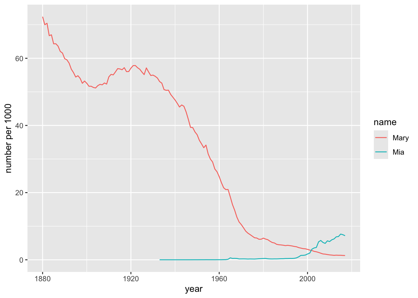
Use the pipe operator and dplyr functions to produce the following graph of the popularity of “Mary” and “Mia” as girl-names over the years. Note that popularity is given as number per one thousand applicants, i.e., as prop * 1000.

9 Lists

11 Strings