3 Functions

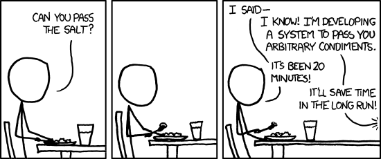
Figure 3.1: The General Problem, by xkcd.

The xkcd cartoon alludes to a common aspiration of programmers: to solve a frequently-occurring problem in general so that we don’t have to keep on devising solutions specific for each case. In R and in most other programming languages, functions are one of the important tools for solving problems in a general manner. In this Chapter we take a close look at how functions work in R. Along the way we’ll learn about environments and scoping, receiving input from the user, and a few more built-in R-functions.

3.1 Motivation for Functions

Suppose you have the job of printing out the word “Kansas” to the console four times, each time on a new line. The code for this is easy enough:

cat("Kansas\n")

## Kansas

cat("Kansas\n")

## Kansas

cat("Kansas\n")

## Kansas

cat("Kansas\n")

## Kansas

Now suppose that you have the job of printing out any given word to the console four times. You could of course, simply copy and paste the above code to a new place in your R script and then change “Kansas” to whatever the desired word is. But that’s an awful lot of work.

You could cut down on the work a bit if you use a variable:

word <- "Kansas"
cat(word, "\n", sep = "")
cat(word, "\n", sep = "")
cat(word, "\n", sep = "")
cat(word, "\n", sep = "")

The advantage of this approach is that, after you copy and paste you only have to make one change, i.e.: substitute the desired word in place of “Kansas” in the assignment to the variable word.

If you were writing a program that involved many four-line print-outs of various words, then you could carry on this way quite a while, producing many similar five-line snippets of printing-code throughout your program.

Eventually it may occur to you that you maybe don’t really need five lines of code. What if cat() supports “vector in, vector out”? If so then we could take advantage of vectorization to obviate the need to repeated calls to `cat().

We could try:

fourWords <- rep("Kansas", 4)
cat(fourWords, "\n")

## Kansas Kansas Kansas Kansas

That just repeats “Kansas” four times, with the default space between in each one—then newline is appended. So we need a newline along with each instance of Kansas.

So instead we try:

fourWords <- rep("Kansas\n", 4)
cat(fourWords)

## Kansas
##  Kansas
##  Kansas
##  Kansas

Not quite what we wanted: cat() inserts the default space at the end of each instance of Kansas\n, resulting in the indentation of lines, 2, 3 and 4.

No problem—let’s just set the separation to the empty string ““:

fourWords <- rep("Kansas\n", 4)
cat(fourWords, sep = "")

## Kansas
## Kansas
## Kansas
## Kansas

Success at last!

If you wanted to implement this new idea throughout your program, you would have to search through the program for the many five-line snippets you created previously, replacing each one of them with the appropriate version of your clever one-liner. Not only is this a lot of work, it’s also quite error-prone: you could miss one or more of the snippets along the way, or on some occasion fail to modify the word within the one-liner to have the value you need at that point.

Accordingly programmers try, as much as possible, to solve problems in a general way and to implement that general solution in one place in their program. Then they call upon that solution in the many different locations where the solution might be required.

Functions are one way in which programmers accomplish this. The following is a function that will print any given word four times, once on each line:

catFourTimes <- function(word) {
  wordWithNewline <- paste(word, "\n", sep = "")
  cat(rep(wordWithNewline, 4), sep = "")
}

Let’s see the function in use:

catFourTimes("Kansas")

## Kansas
## Kansas
## Kansas
## Kansas

It works like a charm! What’s more, once we get to thinking in terms of general solutions, we realize that we might just as well have our function print not only any given word, but print it any given number of times. So instead of catFourTimes() we might actually use the following:

manyCat <- function(word, n) {
  wordWithNewline <- paste(word, "\n", sep = "")
  lines <- rep(wordWithNewline, times = n)
  cat(lines, sep = "")
}

Does it work? Let’s see:

manyCat("Kansas", 5)

## Kansas
## Kansas
## Kansas
## Kansas
## Kansas

Yes indeed!

Let’s consider the advantages of writing functions:

Functions allow us to re-use code, rather than repeating the code throughout our program.
The more generally the functions solves the problem, the varied are the situations in which the function may be re-used.
If we have to change our our approach to the problem—because our original solution was flawed or if there is a need to add new features to our solution, or for any other reason—then we only have to implement the necessary change in the definition of our function, rather than in the many places in the program where the function is actually used.

There is a well-known principle in computer programming called DRY, which is an acronym for “Don’t Repeat Yourself.” Computer code is said to be DRY when general solutions are defined in one place but are usable in many places, and when information needed in many places is defined authoritatively in one place. As a rule, DRY code is easy to develop, debug, read and maintain. The more you get into the habit of expressing solutions to problems in terms of functions, the “drier” your code will be.

3.2 Function Syntax

function is the reserved word in R that permits us to define functions. The general form of a function definition is as follows:

functionName <- function(parameter, parameter, ...) {
  Body of the Function ...
}

functionName is the variable that will refer to the function you define. Like any other identifier, it can contain letters, numbers, the dot and the underscore character, but is not permitted to begin with the dot followed by a number.

After the function reserved word we see a pair of matching parentheses. They contain the parameters of the function, which will be passed into the function as variables referred to by the parameter names.

The body of the function consists of one or more expressions that do the work of the function. Note that the body is enclosed with curly braces. This is only necessary, though, if the body consists of more than one expression. If the body had only one expression then that expression could appear without the braces, like this:

add3 <- function(x) x+3
add3(x = 5)

## [1] 8

add3(-7)

## [1] -4

In the add3() function above, x was a parameter. When the function is called the parameter is assigned a particular value called an argument. We see that add3() was called twice, once with an argument of 3 and again with an argument of -7. If the parameter is explicitly mentioned in the function call, then an equal-sign = separates the parameter and the argument. Note also that the parameter and = may be omitted if it is clear what parameter the argument will be matched to. In the case of add3 there is only one parameter x, so R knows that any value provided within the parentheses is to be assigned to x. R also knows to refer to the order of parameters within the function’s definition to determine which arguments go with which parameters. Thus, the following calls do the same thing:

manyCat(word = "Hello", n = 4)
manyCat(word = "Hello", 4)
manyCat("Hello", n = 4)
manyCat("Hello", 4)
manyCat(n = 4, word = "Hello")

On the other hand, the following would produce an error:

manyCat(4, "Hello")

## NAs introduced by coercion
## Error in rep(wordWithNewline, times = n) :
## invalid 'times' argument

If you don’t label your arguments with the parameters they are to match to, then you must at least write them in the order in which the parameters appear in the definition of the function.

In the definition of functions and in all calls to functions, commas must separate arguments. Thus the following would produce an error:

manyCat("Hello" 4)

## Error: unexpected numeric constant in "manyCat("Hello" 4"

If R cannot match all your arguments to a parameter it will throw an error;

manyCat("Hello", 4, 7)

## Error in manyCat("Hello", 4, 7) : unused argument (7)

You will have noticed by now that parentheses are essential when using a function. What would happen if we typed just the function’s name itself? Give it a try:

manyCat

## function(word, n) {
##   wordWithNewline <- paste(word, "\n", sep = "")
##   lines <- rep(wordWithNewline, times = n)
##   cat(lines, sep = "")
## }

What’s printed to the screen is the code that defines the function. The function itself is not called.

3.2.1 Practice Exercises

Consider the following function:

addThree <- function(n) {
  n +3
}

It adds three to any number you give it. Try it out:

addThree(n = 7)

## [1] 10

What, if anything, is wrong with the following code?
```
addThree(7)
```
What, if anything, is wrong with the following code?
```
addThree(n = 7, x = 5)
```
I’d like to add 3 to the number 15. What, if anything, is wrong with the following code?
```
addThree[15]
```

3.2.2 Solutions to the Practice Exercises

Nothing is wrong. You’ll get a result of 10. You don’t have to use the parameter name n when you call the function: R will figure out that you mean n to be 7.
There will be an error, because when the function was defined there was no parameter x. You can only give a function arguments for parameters that were included in its definition.
addThree is a function. The way you call it is to use parentheses around the arguments, like this: addThree(15). When you use brackets R will assume that you are trying to pick the third element out of a vector named addThree. When it can’t find such a vector, R will throw an error notifying you of that fact.

3.3 What a Function Returns

In this section we learn about return-values of functions.

3.3.1 The Final Expression Evaluated

Let’s write a small function to raise a number to a power:⁷

pow <- function(x,y) {
  x^y
}

Check to see that it works:

pow(2,3)

## [1] 8

All seems well.

If we like we can assign the result of pow() to some variable, for use later on:

a <- pow(2,4)
cat("I have", a, "cats.")

## I have 16 cats.

In computer programming parlance, pow(x, y) is said to return the numerical value x^y: pow(2,3) returns 8, pow(2,4) returns 16, and so on.

In R, what a function returns is: the value of the final expression that it evaluates. You can see this principle at work in the following example:

f <- function(x) {
  2*x + 3
  45
  "hello"
  x^2
}

f(4)

## [1] 16

We put in 4 as the argument for the parameter x, but:

we did not get back 11 (\(2 \times 4 +3\)),
nor did we get back 45,
nor did we get back the string “hello”.

When f() was called, R evaluated all of the expressions in its body, but returned only the value of the final expression it evaluated: \(4^2 = 16\).

In order to understand how functions work in R, you must remember this rule:

In R, a function returns the value of the final expression that it evaluates.

3.3.2 The `return()` Function

R does have a special function to force a function to cease evaluation at a specific point. Its name, unsurprisingly, is return(). Here is an example:

g <- function(x) {
  val <- 3*x +7
  return(val)
  "Hello!"
}

g(1)

## [1] 10

We get \(3*1+7 = 10\), but we don’t get “Hello!”. After returning the 10, the function stopped evaluating expressions: hence it never even bothered to evaluate “Hello”, much less to display it in the console.⁸

It follows that it does not matter whether or not you wrap the final expression of a function in return(). The following two functions do exactly the same thing:

f1 <- function(x) x^2
f2 <- function(x) return(x^2)

Some people—especially those who are familiar with other programming languages where return statements are required—like to wrap the final expression in return(), simply as a matter of clarity.

3.3.3 Writing a “Talky” Function

Suppose that you would like your function to raise a number to a power, returning the answer to the user, but you also want it to print out a message to the console. You might try writing your function like this:

talkySquare <- function(x) {
  result <- x^2
  result
  cat("The square of ", x, " is:  ", result, ".\n", sep = "")
}

We try it out:

talkySquare(4)

## The square of 4 is:  16.

All seems well. But what if we want to save the result in a variable, so that we could perhaps add a number to it later? Something like this, perhaps:

a <- talkySquare(4)

## The square of 4 is:  16.

a + 4

## numeric(0)

The results don’t really make sense. What happened, of course is that R dutifully returned the value of the final expression in the function’s body—the result of the cat() call, not the value of the variable result. If we want both the print-out and the square to be returned, the we have to write our functions like this:

talkySquare <- function(x) {
  result <- x^2
  cat("The square of ", x, " is:  ", result, ".\n", sep = "")
  result
}

This works out as expected:

a <- talkySquare(4)

## The square of 4 is:  16.

a + 4

## [1] 20

Well, maybe it doesn’t work exactly as we would like. It would nice if the function would talk to us only when we ask for the results in the console, not when we are simply assigning the results to a variable for later use. In Chapter 4 we will learn how to make our talky function keep quiet when we prefer silence.

3.3.4 The `print()` Function

Consider the following function:

grumpySquare <- function(x) {
  "OK, OK, I'm getting to it ... "
  x^2
}

We know by now not to expect to see the grumpy message:

grumpySquare(4)

## [1] 16

If we want to see the message, we could wrap it in cat(). Another possibility is to use the print() function:

grumpySquare <- function(x) {
  print("OK, OK, I'm getting to it ... ")
  x^2
}
grumpySquare(4)

## [1] "OK, OK, I'm getting to it ... "

## [1] 16

When R executes a call to print() it is forced to print something out to the console, even if it is in the midst of evaluating expressions in a function. The print-statement is not involved in what the function returns—that’s all up to the final expression that will be evaluated, the expression x^2—but it does cause a result outside of the function itself. Any external result produced by a function (other than what the function returns) is called a side-effect of the function. cat() and print() are examples of functions that, when called inside of some other function, produce side-effects.

You should know that in R you have been calling the print() function quite a bit, without even knowing it. Consider the following line of code:

2+2

## [1] 4

R evaluates the expression 2+2, arriving at the value 4. But what makes the 4 appear on our console? Behind the scenes, R actually evaluated the expression

print(2+2)

That’s what got the 4 into the console! The fact is that whenever you make R evaluate an expression at “top level” (i.e., when you type the expression into the Console) then R will call print() to put the value of the expression into the Console so you can see it.

At this point we don’t use print() explicitly very much—we just rely on R to call it for us when we are evaluating expressions at the console. Later on we will find that it has other uses.⁹

3.3.5 A Function Always Returns a Value

When you call a function, it always returns a value.

Usually it is pretty clear what sort of the value the function returns. For example, the function:

f <- function(x) {
  2 * x + 3
}

returns numbers:

f(7)

## [1] 17

But what is returned by the following function call?

cat("Hello, World!\n")

## Hello, World!

We know that what we see in the console is the intended side-effect of cat(), so it need not be what cat() returned.

In order to find out what cat() returned, we could save the return-value in a variable:

return_value <- cat("Hello, World!\n")

## Hello, World!

Notice that we got the intended side-effect. When we ask R to print the value of return_value, we get:

return_value

## NULL

In fact, cat() always returns the value NULL, which is R’s way of trying to say that it is only used for its side-effect.

Gnerally we use print() only for its side-effect. Does print() also returns NULL? Let’s see:

my_sum <- print(2 + 2)

## [1] 4

my_sum

## [1] 4

Interesting: print() returns the value of the expression that it was aksed to evaluate!

3.3.6 Practice Exercises

What does the following function return?

dog_breeder <- function(dogs) {
  puppies <- dogs + 3
  cat("We now have ", dogs + puppies, " dogs.\n", sep = "")
}

What does the following function return?
```
g <- function(n) {
  n + 3
  "Hello"
}
```
What does the following function return?
```
h <- function(n) {
  "Hello"
  n +3
}
```

3.3.7 Solutions to the Practice Exercises

Like any function, f() returns the value of the last expression that it evaluates. This time the final (and only) expression is the call to cat(). Since cat() always returns NULL, f() always returns NULL, too.
Well, let’s give it a try an see:
```
result <- g(4)
result
```
```
## [1] "Hello"
```
Sure enough, g() returns the value of the last expression that it evaluates. In this case, it’s the expression "Hello".
Like all functions, h() returns the value of the final expression that it evaluates. Hence it will return three more than the value it was given for n.

3.4 Default Values

3.4.1 Madhava’s Approximation of Pi

Sometime around the year 1400CE, the South Indian mathematician Madhava discovered the following infinite-series formula for \(\pi\), the ratio of the circumference to the diameter of a circle:

\[\pi = \frac{4}{1} - \frac{4}{3} + \frac{4}{5} - \frac{4}{7} +\frac{4}{9} - \cdots\] The numerator of each fraction is always 4. The denominators are the odd numbers 1, 3, 5, and so on. The fractions alternate between positive and negative. The idea is that the further you go out in the series, the closer the sum of the fractions will be to \(\pi\). No matter how close you want to get to \(\pi\), you can get that close by adding up sufficiently many of the fractions.

In mathematics courses we learn to write the sum like this:

\[\pi = \sum_{k=1}^{k=\infty} (-1)^{k+1}\frac{4}{2k-1}.\] Here’s how the mathematical notation works:

The \(\Sigma\) sign stands for “sum”: it means that we plan to add up a lot of terms.
The expression \((-1)^k\frac{4}{2k-1}\) after the sum-sign stands for all of the terms that will be added up to make the infinite series.
Underneath the sum-sign, \(k=1\) says that in the expression after the sum sign we will start by letting \(k\) be 1.
If we let \(k=1\), then the expression becomes \[(-1)^2\frac{4}{2 \cdot 1 -1} = \frac{4}{1} = 4,\] the first term in the series.
If we let \(k=2\), then the expression becomes \[(-1)^3\frac{4}{2 \cdot 2 -1} = -\frac{4}{3}\] the second term in the series.
If we let \(k=3\), then the expression becomes \[(-1)^4\frac{4}{2 \cdot 3 -1} = \frac{4}{5}\] the third term in the series.
The \(k = \infty\) above the sum-sign says that we are to keep on going like this, increasing \(k\) by 1 every time, without stopping.
In this way we get the entire infinite series.

What Madhava discovered was that if you do stop after some large number of terms, then the sum of the terms you have constructed will be close to \(\pi\). The more terms you add up before stopping, the closer to \(\pi\) you will get.

Let’s write a function to compute the sum of the first \(n\) terms of the series, where \(n\) can be any value we choose.

# function to approximate pi with Madhava's series
# (sum the first n terms of the series)
madhavaPI <- function(n) {
  # make a vector of all of the k's we need:
  k <- 1:n
  # make a vector of the first n terms of the sum:
  terms <- (-1)^(k+1)*4/(2*k-1)
  # return the sum of the terms:
  sum(terms)
}

R’s vectorization capabilities make it easy to write the code; in fact, the code is essentially a copy of the sum-formula.

Note also the presence of comments in the code above. Anything that appears on a line after the pound-sign # will be ignored by R. We therefore use the #-sign to insert ordinary-language comments into our code in order to explain to others (and to ourselves when we look at the code much later) what we are doing and why we are doing it.

Let’s try it out by adding the first million terms of the series:

madhavaPI(1000000)

## [1] 3.141592

How close is this to \(\pi\)? R has a built-in constant pi that will tell us:

pi

## [1] 3.141593

Madhava’s approximation was pretty close, although we did have to add up quite a few terms!

The madhavaPI() function has a parameter n that stands for the number of terms we want to add up. If we don’t provide a value for n, then there will be an error:

madhavaPI()

## Error in madhavaPI() : argument "n" is missing, with no default

There is a way, though, to allow a user to avoid providing a value for n. We simply provide a default value for it, like this:

madhavaPI <- function(n = 1000000) {
  k <- 1:n
  terms <- (-1)^(k+1)*4/(2*k-1)
  sum(terms)
}

Now we can call the function without having to specify an argument for the parameter n:

madhavaPI()

## [1] 3.141592

The function used the default value of 1000000, so it summed the first million terms.

On the other hand, if the user provides his or her own value for n then the function will override the default:

madhavaPI(100)   # only the first hundred terms, please!

## [1] 3.131593

If you are writing a function for which some of the parameters will often be assigned particular values, it would be a kindness to your users to write in these common values as defaults.

3.4.2 Practice Exercises

Write a function called addSix() that adds six to any number that is given. The function should have a single parameter named x, and the default value of x should be 5.
Tin Man wants to write a function called addTenAndSquare() that takes any given number, adds ten to it and then squares the result. For example, given 5 the function will return \((5 + 10)^2 = 225\). He decides that input value shall be called n and that the default value of n shall be 4. Here is Tin Man’s code:
```
addTenAndSquare <- function(n) {
  n <- 4
  (n + 10)^2
}
```
Has Tin Man accomplished what he set out to do? Why or why not?

3.4.3 Solutions to the Practice Exercises

Here’s the function:

addSix <- function(x = 5) {
  x + 6
}

Let’s test it:

addSix()

## [1] 11

addSix(x = 10)

## [1] 16

Tin Man’s function does not work correctly. Consider the following calls:
```
addTenAndSquare(2)  # should give (2 + 10)^ 2 = 144
```
```
## [1] 196
```
```
addTenAndSquare(5)  # should give (5 + 10)^ 2 = 225
```
```
## [1] 196
```
The function only returns \((4 + 10)^2\),no matter what it is given! The problem is that n is set to 4 within the body of the function. The correct way to define the function would be:
```
addTenAndSquare <- function(n = 4) {
  (n + 10)^2
}
```
This works correctly:
```
addTenAndSquare()
```
```
## [1] 196
```
```
addTenAndSquare(2)
```
```
## [1] 144
```

3.5 Environments and Scope

3.5.1 Environments and Searching

In R an environment is a particular kind of data structure that helps the computer connect names to a value. An environment can be thought of as a bag of names—names for vectors, functions, and all sorts of objects—along with a way (provided automatically by the computer) of getting from each name to the value that it represents. The process that the computer follows in order to connect a name to a value is called scoping. In R, as in many other computer languages, environments are what makes scoping possible. In other words, environments are how R figures out what the names in any piece of code mean.

R has a considerable number of environments—and environments can be created and destroyed throughout the course of an R session—but at any moment only one of them is active. The active environment is the first environment that R will examine when it needs to look up a name in an expression.

The most familiar environment is the Global Environment—the one that is active when you are using R from the console. The names in the Global Environment, along with descriptions of the objects to which they refer, are shown in the Environment panel in the R Studio IDE. Alternatively, you see the names in the active environment by using the ls() function:

ls()

Even better is ls.str(), which will give the name of each object along with a summary of what sort of object it is.

ls.str()

You can remove all of the names from your Global Environment by pressing the Broom icon in the IDE, or by using the rm()function:

rm(list = ls())

As we mentioned previously, the Global Environment is only one of many environments that exist in R. The search() function will show you a number of other environments:

search()

##  [1] ".GlobalEnv"         "package:mosaicData" "package:ggplot2"   
##  [4] "tools:rstudio"      "package:stats"      "package:graphics"  
##  [7] "package:grDevices"  "package:utils"      "package:datasets"  
## [10] "package:methods"    "Autoloads"          "package:base"

search() returns a character vector of names of environments. The first element is the Global Environment itself. The second element is an environment that is associated with last package that R loaded, the third is an environment associated with the next-to-last package, and so on. Each item on the list is considered to be the parent of the environment that came before it. Thus, the Global Environment has a parent environment, a grandparent environment, and so on. The complete sequence of environments is called the search path.

Just as the Global Environment has names for objects, so also the packages have names available for use. When you write code that contains a name, R will search for that name: first in your Global Environment, then in its parent environment—the environment of the last package loaded—and so on until it reaches the final package on the list: package base. If it can’t find the name anywhere, then it will throw an error, telling you that the object “cannot be found.”

Let’s try this with a few examples. First, define a (hopefully) new variable:

quadlingColor <- "red"

Then use it in some code:

cat(quadlingColor, ", white and blue\n", sep ="")

## red, white and blue

R was able to complete your request because:

it found the name `quadlingColor on its search path;
it found the name cat on its search path (and found that it referred to the cat() function)

You can tell where R found these things:

find("quadlingColor")

## [1] ".GlobalEnv"

find("cat")

## [1] "package:base"

R found quadlingColor in the first place it looked, whereas it had to go all the way up to package base to find an object with the name cat that looked like it was the name of a function.

What happens if the same name gets used in two different environments? Let’s investigate. First get a print of cat():

cat

## function (..., file = "", sep = " ", fill = FALSE, labels = NULL, 
##     append = FALSE) 
## {
##     if (is.character(file)) 
##         if (file == "") 
##             file <- stdout()
##         else if (startsWith(file, "|")) {
##             file <- pipe(substring(file, 2L), "w")
##             on.exit(close(file))
##         }
##         else {
##             file <- file(file, ifelse(append, "a", "w"))
##             on.exit(close(file))
##         }
##     .Internal(cat(list(...), file, sep, fill, labels, append))
## }
## <bytecode: 0x7fd580faf208>
## <environment: namespace:base>

I got the definition of the cat() function, all the way up in package base.

Now try:

rep(cat, times = 3)

## Error in rep(cat, times = 3) : 
##   attempt to replicate an object of type 'closure'

I got an error! That’s because the only reference R could find for cat was to the function cat() in package base, and since a function isn’t a vector you can’t repeat it.¹⁰

Next, define a variable named cat:

cat <- "Pippin"

At this point, we the identifier cat appears in at least two environments:

in the Global Environment, where it refers to the string “Pippin”;
in the environment associated with package base, where it refers to the cat()-function.

We can verify the above assertions with find():

find("cat")

## [1] ".GlobalEnv"   "package:base"

Now try:

rep(cat, times = 3)

## [1] "Pippin" "Pippin" "Pippin"

This time it worked! The reason is that R found a character-vector named cat in the Global Environment.

Now try:

cat(cat, "is a cat\n")

## Pippin is a cat

Wait a minute: why did this work? Doesn’t the Global Environment come before package base in the search path? Yes it does, but since the first occurrence of cat was followed by an open parenthesis R expected it to refer to a function. Hence it kept looking along the search path for a function with the name cat, eventually finding our familiar cat() function in package base.

Well then, consider happens if we do this:

cat <- function(...) {
  "Meow!"
}

We have defined a function cat() that returns “Meow!” no matter what it is given as input.¹¹

Now try again:

cat(cat, "is a cat\n")

## [1] "Meow!"

Since the cat() we defined is a function in the Global Environment—which comes before base in the search path—R uses our cat() instead of the base’s cat(). R programmers say that the base version of cat has been masked.

If I want to keep my cat() and still use the base version ofcat() as well, I can do that. In order to be sure of getting a particular package’s version of a function, put the name of the package and then two semicolons before the function-name, like this:

base::cat("This is the good ol' cat() we have been missing!")

## This is the good ol' cat() we have been missing!

But we don’t like our cat() so very much: let’s remove it:

rm(cat)

The vector cat is removed as well by the previous command.

3.5.2 Function Environments

Let’s summarize what we have learned so far:

An environment is a collection of names associated with objects.
The Global Environment is the environment that is active when we are working from the console.
When R needs to look up a name, it consults a search path.
When we are in the Global Environment the search path starts there, and continues to:
- the last package loaded (the parent environment),
- the package before that (the “grandparent environment”),
- and so on …
- … up to package base.
the first object of the right type having the given name that is found along the search path is the object to which R will associate the name.

Just as the Global Environment is a child of the last package loaded, so the Global Environment can have children of its own. In fact a child-environment is created whenever we define a function in the Global Environment and then run it.

Consider the following code:

a <- 10
b <- 4
f <- function(x, y) {
  a <- 5
  print(ls())
  cat("a is ", a, "\n",
      "b is ", b, "\n",
      "x is ", x, "\n",
      "y is ", y, "\n", sep = "")
}

Note that a and b are now in the Global Environment, where the value of a is 10 and the value of b is 5.

We have defined the function f(); pretty soon we will call it. The moment we do so, we will no longer be working directly from the console: instead R will hand control over to the function that it can execute the code in its body. This means that the Global Environment will no longer be the active environment. Instead the active environment will be one that is created at the moment when f is called. Accordingly, it is called the run-time environment (also known as the evaluation environment) of f.

Let’s go ahead and call f():

f(x = 2, y = 3)

## [1] "a" "x" "y"
## a is 5
## b is 4
## x is 2
## y is 3

In the body of the function ls() prints out all of the names in the active environment—which at the moment is the run-time environment of f(). This environment contains a with a value of 5—the a with a value of 10 is masked from it—along with the x and y that were passed into the function as arguments. The a variable having the value 5 that was created within the body of the function is said to be local to the function. Thus we can say that the run-time environment of a function consists of the variables that are local to the function and the arguments that were passed into it.

Observe that b is not a name in the function’s run-time environment: instead it is in the Global Environment. Nevertheless R can “find” b from within the function because the R considers the Global Environment—the environment in which f() was defined—to be the parent of the run-time environment¹², and so the Global Environment is the second place R will look when searching for an object named b. Computer scientists say that b is within the scope of the function.

What happens to the run-time environment when f() finishes executing code? R simply destroys it. It’s as if the a, x and y came to life “inside of” f() but died as soon as f() stopped working.

The next time f() is called, a new run-time environment will be created to enable the code in the body of f() to do its work.

One consequence of the ephemeral nature of run-time environments is that they are not accessible from parent environments. Thus if the active environment is the Global Environment and you run across a reference to a, you will never “find” the a “inside of” f() or “inside of” any other function, for that matter. R looks only in the active environment and in ancestor-environments, never in child-environments, and anyway the run-time environment no longer exists after a function has been called.

Let’s make sure of this with an example.

a <- 5
f <- function() {
  a <- 10
  print(ls.str()) # print out the active environment
}
f()

## a :  num 10

Did calling f() change the value of a in the Global Environment? Let’s see:

## [1] 5

Nope, a is still 10.

This is a very good thing. It would be very confusing if assignment to a variable within a function were to “change the values” of variables—happening to have the same name—that were declared outside of the function’s environment.

3.5.3 Practice Exercises

Starting from a new R session and an empty Global Environment, I run the following code:
```
m <- 5
f <- function(n) {
  m <- 10
  a <- m + 5
  n^2
}
```
What two items are now in my Global Environment?
I then run the following code:
```
g <- f(10)
```
What items are now in my Global Environment? What is the value of g? What is the value of m?
When f() was called, a runtime environment was created for it. By the time it got down to the line n^2, what items were in that environment, and what were their values?

3.5.4 Solutions to the Practice Exercises

There are now two items in the Global Environment:
- m: its value is 5
- f, the fuunction I defined.
Now there are three items in the Global Environment:
- m: its value is still 5. (The m in the runtime environment is not in the “scope” of the Global Environment.)
- f, the fuunction I defined is still there.
- I also have g: its value is \(10^2 = 100\).
The items in the runtime environment were:
- the parameter n, with a value of 10;
- m, with a value of 10;
- a, with a value of 15.

3.6 More to Learn

By now we have have:

learned about vectors, an important data structure in R;
met quite a few R functions that help us manipulate vectors and print things to the console;
learned how to write functions so that we can re-use solutions to problems.

But still it seems that—unless we can find a clever way to exploit vectorization—R isn’t doing anything very impressive, really. In order to unlock the true powers of R (or any programming language, for that matter) we have to acquire more control over what expressions R will evaluate, how many times it will evaluate them, and under what conditions it will do so. This is the domain of flow control, the subject of our next chapter.

3.7 More in Depth

3.7.1 Argument-Matching

Sometimes you will see functions in R that provide what appears to be a vector of default values. You’ll see this in the following example, which concerns a function that uses a named vector to report the favorite color of each of the major groups of inhabitants of the Land of Oz.

inhabitants <- c("Munchkin", "Winkie", 
            "Quadling", "Gillikin")
favColor <- c("blue", "yellow", "red", "purple")
names(favColor) <- inhabitants

favColorReport <- function(inhabitant = inhabitants) {
  x <- match.arg(inhabitant)
  cat(favColor[x],"\n")
}

Here are a couple of sample calls:

favColorReport("Winkie")

## yellow

favColorReport("Quadling")

## red

It might get tiresome to type out the full name of each group of inhabitants. What would happen if we got a bit lazy?

favColorReport("Win")

## yellow

favColorReport("Wi")

## yellow

favColorReport("W")

## yellow

favColorReport("Qua")

## red

favColorReport("Gil")

## purple

The key to this behavior is two-fold:

The vector inhabitants was set as the “default value” of the parameter inhabitant.
We called the match.arg() function, which found the element of inhabitants that matched what the user actually submitted for the parameter inhabitant. This element was then assigned to x, and we used x to report the desired color.

Sometimes when you look at R-help you’ll see the default value for a parameter set as a vector—usually a character-vector, as in our example. Most likely what is going on is that somewhere inside the function R will attempt to match the argument you provide with one of the elements of that “default” vector. When a function is written in this way, the possible parameters can have quite long names but the user doesn’t have to type them in all the way, as long as the user types enough characters to pick out uniquely an element of the default vector.

The matching is done by exact match of initial characters. For example, it won’t do for me to enter:

favColorReport("w")  # wants Winkies, but using lower-case w

## Error in match.arg(inhabitant) : 'arg' should be one of 
## “Munchkin”, “Winkie”, “Quadling”, “Gillikin”

Note that the default vector isn’t really a default value for the parameter. Its first element does, however, serve as the default value:

favColorReport()  # defaults to "Munchkin"

## blue

3.7.2 A Note on Parameters vs Arguments

It’s important to keep in mind the distinction between a parameter of a function on the one hand and, on the other hand the argument that gets supplied to that parameter.

When you are just starting out in R programming, this distinction can be difficult to remember, especially when the parameter and the argument have the same name. Now that we understand environments, though, we can get a grip on this tricky situation.

Let’s proceed by way of an example.

First of all, clear out your Global Environment:

rm(list = ls())

Next make a simple function that adds three to any given number. Our function will take one parameter n (the number to which 3 is to be added), and the default value of n shall be 4.

addThree <- function(n = 4) {
  n + 3
}

Next, bind the name n to the value 2:

n <- 2

You should now have two items in your Global Environment. Confirm this:

ls.str()

## addThree : function (n = 4)  
## n :  num 2

Now call the function as follows:

addThree(n = 5)

## [1] 8

Let’s recall how this works:

R sees that you want to assign the value 5 to the parameter n.
R executes the code in the body of the function. All is well.

Now call the function as follows:

addThree()

## [1] 7

Let’s recall how this works:

R sees that you did not assign anything to the parameter n.
“That’s OK”, says R. “I’ll use the default value of 4 for n.”
R executes the code in the body of the function. All is well.

Next, call the function as follows:

addThree(n = n)

## [1] 5

Let’s think about how this works:

R sees that you want to assign something to the parameter n. Apparently it is the value of a name n in some environment.
“Fine”, says R. “I’ll look up the value of this n thingie, if ever I have to use it in a computation.”
R executes the one line of code in the body of the function.
“Well, I’ll be darned,” says R, “I do need the value of this n thingie after all. I’ll look it up.”
R looks for n, finding it in the Global Environment. Apparently it’s bound to 2.
R computes \(2+3\) and returns \(5\). All is well.

Now call the function as follows:

addThree(n)

## [1] 5

Again let’s consider how this works:

R sees the n. Since the function has only one parameter, R figures that you mean to assign the value of n (in some environment) to its parameter n.
Everything now proceeds just as before, with 5 being the number returned.

Now let’s remove n from the Global Environment:

rm(n)

Now call the function again, in the following way:

addThree(n = n)

Error in addThree(n = n) : object 'n' not found

Can you see why we got an error? This time when R goes looking for n, it can’t find it: n is no longer in the Global Environment, nor is it anywhere else along the search path. Accordingly R throws the error.

The call addThree(n) will elicit the same error message, for the same reason.

The moral of the story is:

Parameters are NOT the same thing as arguments, even when a parameter and an argument happen to be called by the same name.

3.7.3 More About Packages

We have seen that packages make up most of the search path when the active directory is the Global Environment. We have also mentioned a couple of packages explicitly—mosaicData and ggplot2 back in Section 1.6 for example. But what exactly is a package?

A package is a bundle of R-code (usually functions) and data that is organized according to well-defined conventions and documented so that users can learn how to use the code and data. When someone bundles code into a package it becomes easy to share it with others and and to re-use it for one task after another.

3.7.3.1 Installed Packages

When you click on the Packages tab in the lower right-hand pane in R Studio, you can see a list of all the packages that are installed on the machine. You can get the same information by running the command:

installed.packages()[, c("Package", "Version")]

In fact R is really nothing but a collection of packages. Many of the R-functions you have been learning about come from the package base. This is one of a number of packages that are automatically attached to the search path when an R session begins. Other packages have to be attached by you if you want immediate access to all of the functions and data that they contain.

In order to attach a package, you can click the little box next to its name in the Package tab in R-Studio, or you can attach it from the console with the command:

library(<name of package here>)

When you don’t want a package any more, you can detach it from the search path by un-clicking the little box, or by running this command:

detach("package:<name of package here>", unload=TRUE)

The package will still be installed, ready to be attached whenever you like.

3.7.3.2 Learning About a Package

You can learn about a Package by clicking on its name, or by using the command:

help(<name of package>)

From the display that shows in the Help pane you can navigate to learn about each of the functions and data sets that come with the package.

3.7.3.3 Installing Packages

You can also install additional packages on the computer. This can be done by clicking the Install button in R Studio and typing in the package name, or with the command:

install.packages("<name of package here>")

The package will be downloaded from the Comprehensive R Archive Network (CRAN) and installed in in your Home directory.

As long as we are working on the R Studio server, it’s a good idea to refrain from installing packages yourself, unless they are packages that we don’t use in class and that you simply want to explore on your own. That’s because when you install your own packages on the Server they go into a special directory in your Home folder and become part of your “User Library”. Packages that are installed by a system administrator for general use are in the “System Library.” If a package is in your User Library and in the System Library, when you ask to attach it you will get the version that it is your User Library. Now packages are updated from time to time, so it may happen that the version you have in your User Library will be different from the one in the System Library. If that is the case then your package might not work the same way for you as it does for the instructor and for other students: that can be confusing.

Eventually, though, you will install R and R Studio on your own computer, and then you will have to install many packages on your own.

Not all packages come from CRAN: many useful packages exist on other repositories, including the very popular code repository known as GitHub. Special functions exist to install R-packages from GitHub. For example, you may eventually wish to install the package tigerData, which resides in a GitHub repository belonging to your instructor. In order to install it, you would use the install_github() function from the devtools package (Pruim, Kaplan, and Horton 2022), like this:

devtools::install_github(repo = "homerhanumat/tigerData")

There are a couple of things worth noting about the command above:

The argument to repo has two parts: the word before the “/” is the username of the individual who owns the repository; the word after the “/” is the name of the repository itself. For R-packages on GitHub, the name of the repository is the same as the name of the package.
The double-colon :: is used to access a function from a package, without having to attach the entire package. Thus devtools::install_github() refers to the function install_github() in package devtools. Similarly, if you want to access, say, just the Births78 data set from the mosaicData package then you could refer to it as mosaicData::Births78.

The Main Ideas of This Chapter

You can write your own R-function with the reserved word function and the proper syntax.
In R, a function returns the value of the final expression that it evaluates.
When you write a function, you can give one or more of its parameters a default value. When the function is called without assigning a value to the parameter, its default value is used. But when the user calls the function with a different value assigned to the parameter, R will use that value—not the default.
When you write a new R-function, don’t just start typing the code for the function. Instead work slowly and systematically, using the five-step procedure that we practice in class:
1. Know the specs. Understand the specifications for the function: what its parameters should be called, what it needs to do, and how it needs to return its result.
2. Solve for an example. Write a program does the required work of the function, for a specific example. The program should be written generally, so that it would work on any other example. It is good practice to give your example(s) the same name(s) you plan to use for the parameter(s) in your function.
3. Write the function, encapsulating the work of your program into the body of your function.
4. Test your function by calling it on various examples, until you are sure that it works properly.
5. As a final check, consult the specs one more time.
When R has to evaluate an expression, it uses the search path to find the values associated with names in that expression. The search path always starts with the active environment.
When you call a function is called in R, a special temporary environment called the run-time environment for the function is created, and this becomes the active environment until the function finishes. The parent environment of the run-time environment of a function is the environment in which the function was defined.
You can learn a lot about how a function does its work by running it in the debugger, as we often do in class. Try this for any function you want to understand better.

Links to Class Slides

Quarto Presentations that I sometimes use in class:

Glossary

Don’t Repeat Yourself (DRY): A principle of computer programming that holds that general solutions should be set forth in one place and usable in many places, and that information needed in many places should be defined authoritatively in one place.
Parameters of a Function: The parameters of a function (also called the formal arguments of the function) are the names that will be used in the body of the function to refer to the actual arguments supplied to the function when it is called.
Argument: An argument for a function is a value that is assigned to one of the parameters of the function. (Sometimes arguments are called an actual arguments in order to distinguish then from parameters that are often called formal arguments.)

“It’s useful to distinguish between the formal arguments and the actual arguments of a function. The formal arguments are a property of the function, whereas the actual or calling arguments can vary each time you call the function.”

—H. Wickham, Advanced R Programming

Body of a Function: The body of a function is the code that is executed when the function is called. In R, when the body consists of more than one expression then it appears inside of curly braces.
Side-Effect: Any result produced outside of the run-time environment of a function, other than the value that the function returns.
Default Value: A value for a parameter of a function that is provided when the function is defined. This value will become the value assigned to the parameter when the function is called, unless the user explicitly assigns some other value as the argument.
Environment: An object stored in the computer’s memory that keeps track of name-value pairs.
Active Environment: The environment that R will consult first in order to find the value of any name in an expression.
Global Environment: The environment that is active when one is using R from the console.
Parent Environment: The second environment (after the active environment) that R will search when it needs to look up a name.
Run-time Environment (also called the “Evaluation Environment”): A special environment that is created when a fuction is called and ceases to exist when the function finishes executing. It contains the values that are local to the function and the arguments of the function as well.
Scoping: The process by which the computer looks up the object associated with a name in an expression.
Search Path: The sequence of environments that the computer will consult in order to find an object associated with a name in an expression. The sequence begins with the active environment, followed by its parent environment, followed by the parent of the parent environment, and so on.
Package: A bundle of R-code and data that is organized according to well-defined conventions and documented so that users can learn how to use the code and data.

Exercises

Write a function called pattern() that when given a character will print out the character in a pattern like this:
```
*
**
***
**
*
```
That is: a row of one, then a row of two, then a row of three, then a row of two, and finally a row of one.

The function should take one parameter called char. The default value of this parameter should be *. Typical examples of use should be as follows:
```
pattern()
```
```
## *
## **
## ***
## **
## *
```
```
pattern(char = "x")
```
```
## x
## xx
## xxx
## xx
## x
```
Write a function called charSquare() that when given two characters will use them to make a square like this:
```
****
a  a
a  a
****
```
That is: a row of four of one of the characters, then two rows that consist of the other character followed by two spaces followed by that other character, and finally a row of four of the first character.

The function should take two parameters called end and middle. The default value of end should should be * and the default value of middle should be x. Typical examples of use should be as follows:
```
charSquare()
```
```
## ****
## x  x
## x  x
## ****
```
```
charSquare(end = "z", middle = "%")
```
```
## zzzz
## %  %
## %  %
## zzzz
```
Write a function called reverse() that, given any vector, returns a vector with the elements in reverse order. It should take one parameter called vec. The default value of vec should be the vector c("Bob", "Marley"). Typical examples of use should be:
```
reverse()
```
```
## [1] "Marley" "Bob"
```
```
reverse(c(3,2,7,6))
```
```
## [1] 6 7 2 3
```
Hint: Recall how you can use sub-setting to reverse:
```
firstFiveLetters <- c("a", "b", "c", "d", "e")
firstFiveLetters[5:1]
```
```
## [1] "e" "d" "c" "b" "a"
```
You just need to figure out how to reverse vectors of arbitrary length.

Note: It so happens that R already provides a function rev() that reverses the elements of a given vector, but your assignment is to write your own function that reverses vectors. In particular, you may not use rev() in the body of your reverse() function!
A vector is said to be a palindrome if reversing its elements yields the same vector. Thus, c(3,1,3) is a palindrome, but c(3,1,4) is not a palindrome.

Write a function called isPalindrome() that, when given any vector, will return TRUE if the vector is a palindrome and FALSE if it is not a palindrome. The function should take a single parameter called vec, with no default value. Typical examples of use should be:
```
isPalindrome(vec = c("Bob", "Marley", "Bob"))
```
```
## [1] TRUE
```
```
isPalindrome(c(3,2,7,4,3))
```
```
## [1] FALSE
```
Hint: You already have the function reverse() from the previous Exercise. Use this function, along with the Boolean operator == and the all() function.
The eighteenth-century mathematician Leonhard Euler discovered that:

\[\frac{\pi^2}{6} = \sum_{k=1}^{k=\infty} \frac{1}{k^2}.\] It follows that \[\pi = \sqrt{\left(\sum_{k=1}^{k=\infty} \frac{6}{k^2}\right)}.\] Use this fact to write a function called eulerPI() that will approximate \(\pi\). The function should take a single parameter n, which is the number of terms in the infinite series that are to be summed to make the approximation. The default value of n should be 10,000.
Consider the infinite series:

\[\sum_{k=1}^{k=\infty} \frac{1}{k(k+1)}.\] Write a function called partialSum() that will compute the sum of the first \(n\) terms of this series. The function should take a single parameter n, which is the number of terms in the series that are to be summed to make the approximation. The default value of n should be 10,000. Use the function to compute the sum of the first 10,000 terms and the sum of the first 100,000 terms. What number do you thnk the series converges to?

2 Vectors

4 Flow-Control

3 Functions

3.1 Motivation for Functions

3.2 Function Syntax

3.2.1 Practice Exercises

3.2.2 Solutions to the Practice Exercises

3.3 What a Function Returns

3.3.1 The Final Expression Evaluated

3.3.2 The return() Function

3.3.3 Writing a “Talky” Function

3.3.4 The print() Function

3.3.5 A Function Always Returns a Value

3.3.6 Practice Exercises

3.3.7 Solutions to the Practice Exercises

3.4 Default Values

3.4.1 Madhava’s Approximation of Pi

3.4.2 Practice Exercises

3.4.3 Solutions to the Practice Exercises

3.5 Environments and Scope

3.5.1 Environments and Searching

3.5.2 Function Environments

3.5.3 Practice Exercises

3.5.4 Solutions to the Practice Exercises

3.6 More to Learn

3.7 More in Depth

3.7.1 Argument-Matching

3.7.2 A Note on Parameters vs Arguments

3.7.3 More About Packages

3.7.3.1 Installed Packages

3.7.3.2 Learning About a Package

3.7.3.3 Installing Packages

The Main Ideas of This Chapter

Links to Class Slides

Glossary

Exercises

3.3.2 The `return()` Function

3.3.4 The `print()` Function