Using qnormGC()
Comparison of qnormGC() with pnormGC()
The function pnorm() in regular R, as well as the function pnormGC() in thetigerstats` package, compute probabilities from known bounding values. For example, suppose that \(X\) is a normally distributed random variable with mean 70 and standard deviation 3, and that you want to know:
\[P(X < 72).\]
Then you know the boundary value 72, but you don’t know the probability: the area under the normal density curve before 72. Functions like pnormGC() aim to give you that area–that probability:
pnormGC(72, region="below", mean=70,
        sd=3,graph=TRUE)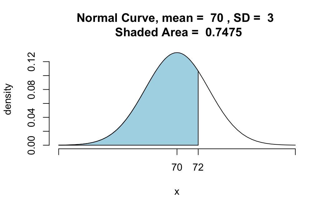
## [1] 0.7475075The function qnormGC()aims to do the opposite: given an area, find the boundary value that determines this area.
For example, suppose you want to find that 85th percentile of a normal distribution whose mean is 70 and whose standard deviation is 3. Then you ask for:
qnormGC(0.85,region="below",mean=70,sd=3)## [1] 73.1093The value 73.1093 is indeed the 85th percentile, in the sense that 85% of the values in a population that is normally distributed with mean 70 and standard deviation 3 will lie below 73.1093. In other words, if you were to pick a random member \(X\) from such a population, then
\[P(X < 73.1093) = 0.85\].
Quite often you will want to check your understanding by making a graph of the known percent, with the bounding percentile on the x-axis:
qnormGC(0.85,region="below",mean=70,sd=3,graph=TRUE)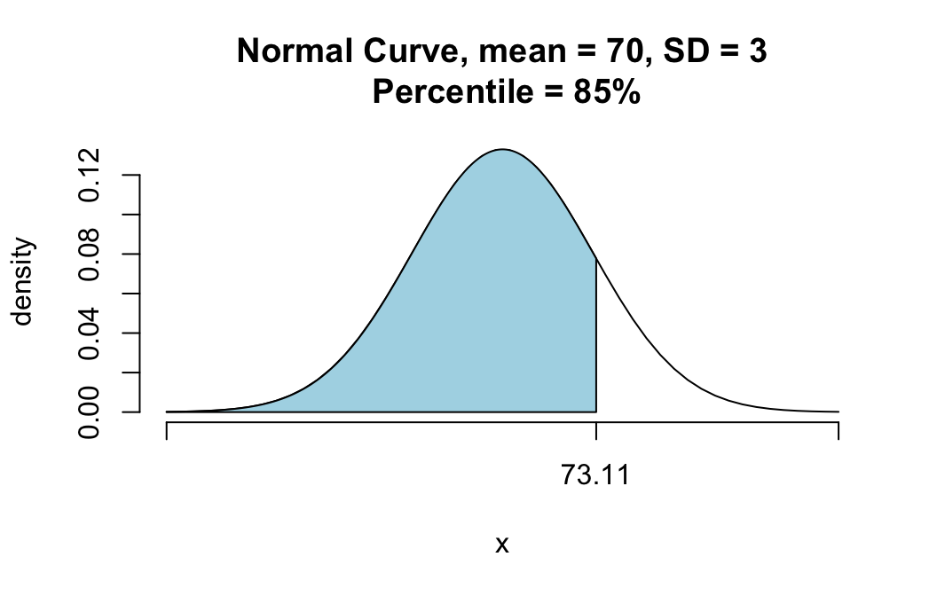
## [1] 73.1093A Few More Examples
Making the Top Ten Percent (An Area Above)
Suppose that SAT scores are normally distributed, and that the mean SAT score is 1000, and the standard deviation of all SAT scores is 100. How high must you score so that only 10% of the population scores higher than you?
Here’s the solution: just set region to “above”:
qnormGC(0.10,region="above",mean=1000,sd=100,graph=TRUE)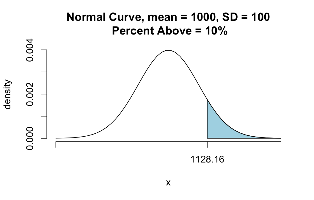
## [1] 1128.155In other words, the 90th percentile of SAT scores is around 1128.
Of course, you could have got the same thing by realizing that when 10% are above, 90% are below. Then you could just ask for:
qnormGC(0.90,region="below",mean=1000,sd=100)## [1] 1128.155An Area Between
Find a positive number \(z\) so that the area under the standard normal curve between \(-z\) and \(z\) is 0.95.
Here, we can set the region argument to “between”. The default value for mean is 0 and for sd the default is 1, so we can leave those arguments out if we like:
qnormGC(0.95,region="between",graph=TRUE)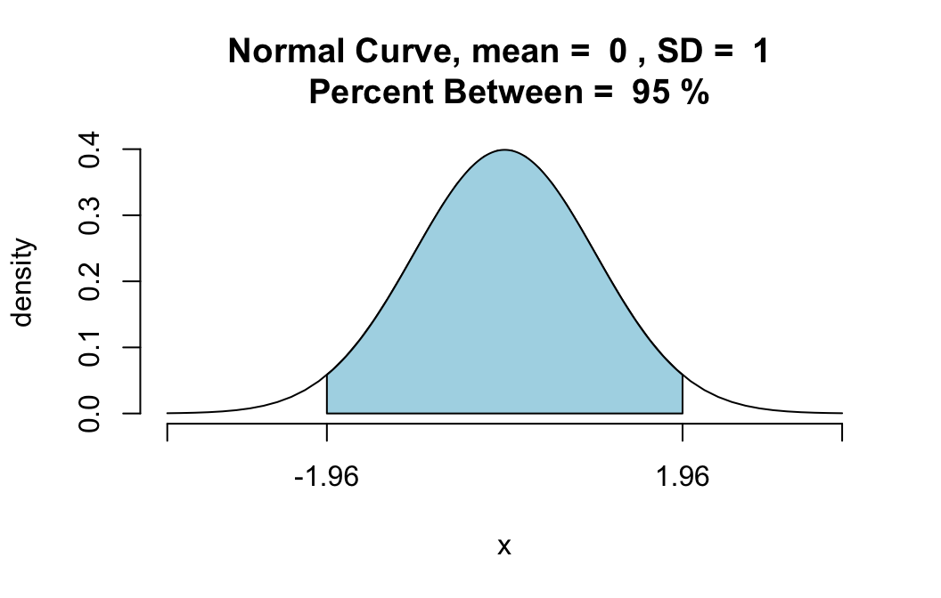
## [1] -1.959964 1.959964Both bounds are given. The positive number we sought is about 1.96.
An Area Outside
Find a positive number \(z\) so that the area under the standard normal curve before \(-z\) plus the area after \(z\) is 0.10.
Here, we can set the region argument to “outside”. The default value for mean is 0 and for sd the default is 1, so we can leave those arguments out if we like:
qnormGC(0.10,region="outside",graph=TRUE)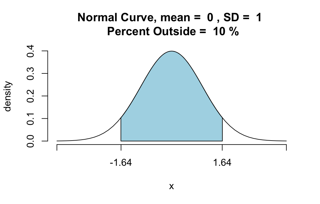
## [1] -1.644854 1.644854Both bounds are given. The positive number we sought is about 1.645.