Using chisqtestGC()
Preliminaries
You use the \(\chi^2\)-test when you are addressing the inferential aspect of research questions about:
- the relationship between two factor variables (test for association);
- the distribution of one factor variable (goodness-of-fit test).
Two Factor Variables (Association)
Formula-Data Input
When your data are in raw form, straight from a data frame, you can perform the test using “formula-data input”. For example, in the mat111survey data, we might wonder whether sex and seating preference are related, in the population from which the sample was (allegedly randomly) drawn. The function call and the output are as follows:
chisqtestGC(~sex+seat,data=m111survey)## Pearson's Chi-squared test
##
## Observed Counts:
## seat
## sex 1_front 2_middle 3_back
## female 19 16 5
## male 8 16 7
##
## Counts Expected by Null:
## seat
## sex 1_front 2_middle 3_back
## female 15.21 18.03 6.76
## male 11.79 13.97 5.24
##
## Contributions to the chi-square statistic:
## seat
## sex 1_front 2_middle 3_back
## female 0.94 0.23 0.46
## male 1.22 0.29 0.59
##
##
## Chi-Square Statistic = 3.734
## Degrees of Freedom of the table = 2
## P-Value = 0.1546Two-Way Table Input
Sometimes you already have a two-way table on hand:
SexSeat <- xtabs(~sex+seat,data=m111survey)
SexSeat
## seat
## sex 1_front 2_middle 3_back
## female 19 16 5
## male 8 16 7In that case you can save yourself some typing by entering the table in place of the formula and the data arguments:
chisqtestGC(SexSeat)A Table From Summary Data
Remember: if you are given summary data, only, then you can construct a nice two-way table and enter it into chisquaretestGC(). Suppose that you want this two-way table:
| Front | Middle | Back | |
|---|---|---|---|
| Female | 19 | 16 | 5 |
| Male | 8 | 16 | 7 |
You can get it as follows:
MySexSeat <- rbind(female=c(19,16,5),male=c(8,16,7))
colnames(MySexSeat) <- c("front","middle","back")Let’s just check to see that this worked:
MySexSeat## front middle back
## female 19 16 5
## male 8 16 7Then you can enter MySexSeat into the function:
chisqtestGC(MySexSeat)Simulation
When the Null’s expected counts are low, chisqtestGC() delivers a warning and suggests the use of simulation to compute the \(P\)-value. You do this by way of the argument simulate.p.value, and you have three options:
simulate.p.value = "fixed"simulate.p.value = "random"simulate.p.value = "TRUE"
Explanatory Tallies Fixed
Suppose that the objects under study are not a random sample from some larger population, and that the way chance comes into the production of the data is through random variation in all of the other factors—besides the explanatory variable— that might be associated with the response variable. Then since the items being observed are fixed, the tally of values for the explanatory variable are fixed. The response values for these items are the product of chance, but only through random variation in those other factors.
The study from the ledgejump data frame was an example of this. The 21 incidents were fixed, so there were nine cold-weather incidents and 12 warm-weather incidents, no matter what. The crowd behavior at each incident, however is still a matter of chance.
In such a case you might want to resample under the restriction that in all of your resamples, the tally for the explanatory variable stays just the same as it was in the data you observed. Then your function call looks like:
chisqtestGC(~weather+crowd.behavior,data=ledgejump,
simulate.p.value="fixed",B=2500)## Pearson's chi-squared test with simulated p-value, fixed row sums
## (based on 2500 resamples)
##
## Observed Counts:
## crowd.behavior
## weather baiting polite
## cool 2 7
## warm 8 4
##
## Counts Expected by Null:
## crowd.behavior
## weather baiting polite
## cool 4.29 4.71
## warm 5.71 6.29
##
## Contributions to the chi-square statistic:
## crowd.behavior
## weather baiting polite
## cool 1.22 1.11
## warm 0.91 0.83
##
##
## Chi-Square Statistic = 4.0727
## Degrees of Freedom of the table = 1
## P-Value = 0.05You can set B, the number of resamples, as you wish, but it should be at least a few thousand. Of course the \(P\)-value, having been determined by random resampling, will vary from one run of the function to another.
Explanatory Tallies Random
In the m111survey study on sex and seating preference, the subjects are a random sample from a larger population. In that case the tallies for both the explanatory and the response variables depend upon chance. If you simulate in such a case, then you set simulate.p.value to “random”:
chisqtestGC(~sex+seat,data=m111survey,
simulate.p.value="random",B=2500)## Pearson's chi-squared test with simulated p-value, marginal sums not fixed
## (based on 2500 resamples)
##
## Observed Counts:
##         seat
## sex      1_front 2_middle 3_back
##   female      19       16      5
##   male         8       16      7
##
## Counts Expected by Null:
## seat
## sex 1_front 2_middle 3_back
## female 15.21 18.03 6.76
## male 11.79 13.97 5.24
##
## Contributions to the chi-square statistic:
## seat
## sex 1_front 2_middle 3_back
## female 0.94 0.23 0.46
## male 1.22 0.29 0.59
##
##
## Chi-Square Statistic = 3.734
## Degrees of Freedom of the table = 2
## P-Value = 0.1687Both Tallies Fixed
If you want to resample in such a way that the tallies for BOTH the explanatory and response variables stay exactly the same as they were in the actual data, then you set simulate.p.value to “TRUE”. This invokes R’s standard method for resampling:
chisqtestGC(~sex+seat,data=m111survey,
             simulate.p.value=TRUE,B=2500)
## Pearson's chi-squared test with simulated p-value
## (based on 2500 resamples)
##
## Observed Counts:
## seat
## sex 1_front 2_middle 3_back
## female 19 16 5
## male 8 16 7
##
## Counts Expected by Null:
## seat
## sex 1_front 2_middle 3_back
## female 15.21 18.03 6.76
## male 11.79 13.97 5.24
##
## Contributions to the chi-square statistic:
## seat
## sex 1_front 2_middle 3_back
## female 0.94 0.23 0.46
## male 1.22 0.29 0.59
##
##
## Chi-Square Statistic = 3.734
## Degrees of Freedom of the table = 2
## P-Value = 0.1704It’s not easy to understand why R would adopt such a method, but there is some good theoretical support for it. If you are ever in doubt about how to simulate, just use this third option.
Graphs of the P-Value
You can get a graph of the \(P\)-value in the plot window by setting the argument graph to TRUE. When you did not simulate, the graph shows a density curve for the \(\chi^2\) random variable with the relevant degrees of freedom. When you simulate, the graph is a histogram of the resampled \(\chi^2\)-statistics.
Here is a case with no simulation:
chisqtestGC(~sex+seat,data=m111survey,graph=TRUE)## Pearson's Chi-squared test
##
## Observed Counts:
## seat
## sex 1_front 2_middle 3_back
## female 19 16 5
## male 8 16 7
##
## Counts Expected by Null:
## seat
## sex 1_front 2_middle 3_back
## female 15.21 18.03 6.76
## male 11.79 13.97 5.24
##
## Contributions to the chi-square statistic:
## seat
## sex 1_front 2_middle 3_back
## female 0.94 0.23 0.46
## male 1.22 0.29 0.59
##
##
## Chi-Square Statistic = 3.734
## Degrees of Freedom of the table = 2
## P-Value = 0.1546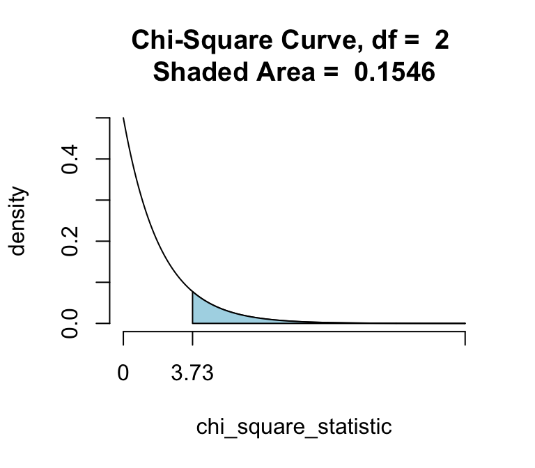
Graph of P-value, no simulation
Here is a case with simulation:
chisqtestGC(~sex+seat,data=m111survey,
             simulate.p.value="random",B=2500,graph=TRUE)
## Pearson's chi-squared test with simulated p-value, marginal sums not fixed
## (based on 2500 resamples)
##
## Observed Counts:
## seat
## sex 1_front 2_middle 3_back
## female 19 16 5
## male 8 16 7
##
## Counts Expected by Null:
## seat
## sex 1_front 2_middle 3_back
## female 15.21 18.03 6.76
## male 11.79 13.97 5.24
##
## Contributions to the chi-square statistic:
## seat
## sex 1_front 2_middle 3_back
## female 0.94 0.23 0.46
## male 1.22 0.29 0.59
##
##
## Chi-Square Statistic = 3.734
## Degrees of Freedom of the table = 2
## P-Value = 0.1575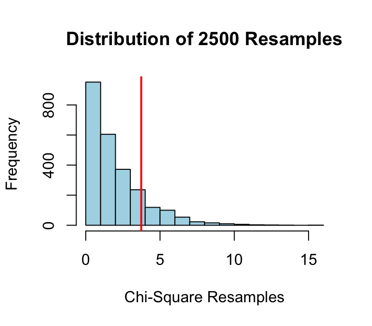
Graph of P-value, with simulation
One Factor Variable (Goodness of Fit)
Formula-Data Input
The variable seat in the m111survey data frame indicates the classroom seating preference of each person in the survey. Suppose we want to know whether or not the sample data provide strong evidence that seating preference in the Georgetown College population is not uniformly distributed among the three possible options (Front, Middle, and Back). That is, letting
\(p_f =\) proportion of all GC students who prefer the front,
\(p_m =\) proportion of all GC students who prefer the middle,
\(p_b =\) proportion of all GC students who prefer the back,
we want to test the hypotheses:
\(H_0:\) \(p_f = 1/3\) and \(p_m = 1/3\) and \(p_b = 1/3\)
\(H_a:\) at least one of the above proportions is not \(1/3\)
We can do so using the \(\chi^2\)-test for goodness of fit. The argument p will give what the Null Hypothesis believes to be the distribution of the variable seat in the Georgetown College population:
chisqtestGC(~seat,data=m111survey,
            p=c(1/3,1/3,1/3),
            graph=TRUE)
## Chi-squared test for given probabilities
##
## Observed counts Expected by Null Contr to chisq stat
## 1_front 27 23.67 0.47
## 2_middle 32 23.67 2.93
## 3_back 12 23.67 5.75
##
##
## Chi-Square Statistic = 9.1549
## Degrees of Freedom of the table = 2
## P-Value = 0.0103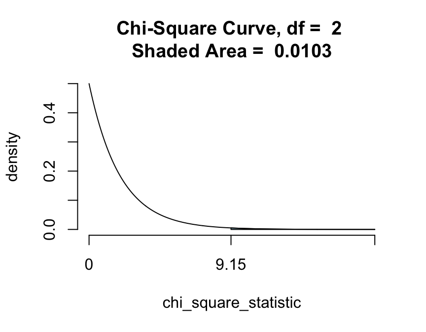
Summary Data
Suppose that the data had only come to us in summary form:
| Front | Middle | Back |
|---|---|---|
| 27 | 32 | 12 |
We could still perform the test, by making a table and storing it as an R-object:
Seat <- c(front=27,middle=32,back=12)
Seat
## front middle back
## 27 32 12Then we could perform the test using Seat:
chisqtestGC(Seat,p=c(1/3,1/3,1/3))## Chi-squared test for given probabilities
##
## Observed counts Expected by Null Contr to chisq stat
## front 27 23.67 0.47
## middle 32 23.67 2.93
## back 12 23.67 5.75
##
##
## Chi-Square Statistic = 9.1549
## Degrees of Freedom of the table = 2
## P-Value = 0.0103Simulation
When expected cell counts fall below 5, chisqtestGC() issues a warning and suggests the use of simulation. We can perform simulation at any time, though.
For goodness-of-fit tests, the only relevant form of simulation is the one provided by setting simulate.p.value to TRUE. Of course we also need to set the number B of resamples.
set.seed(678910)
chisqtestGC(~seat,data=m111survey,
            p=c(1/3,1/3,1/3),
            simulate.p.value=TRUE,
            B=2500,graph=TRUE)
## Pearson's chi-squared test with simulated p-value
## (based on 2500 resamples)
##
## Observed counts Expected by Null Contr to chisq stat
## 1_front 27 23.67 0.47
## 2_middle 32 23.67 2.93
## 3_back 12 23.67 5.75
##
##
## Chi-Square Statistic = 9.1549
## Degrees of Freedom of the table = 2
## P-Value = 0.0116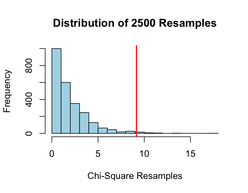
Want Less Output?
If you do not wnat to see quite so much output to the console and are only interested in the essentials for reporting a \(\chi^2\)-test, then set the argument verbose to FALSE:
chisqtestGC(~sex+seat,data=m111survey,
            verbose=FALSE)
## Pearson's Chi-squared test
##
## Chi-Square Statistic = 3.734
## Degrees of Freedom of the table = 2
## P-Value = 0.1546