Using proptestGC()
Preliminaries
You use proptestGC() for inferential procedures regarding:
- one population proportion \(p\);
- the difference of two population proportions, \(p_1 - p_2\).
The function comes from the tigerstats package, so make sure that tigerstats is loaded:
require(tigerstats)One Proportion, From Data Frame (Read This!!)
In inference procedures regarding one proportion, binomtestGC() is preferred over proptestGC(), especially at smaller sample sizes. Nevertheless, read this section carefully. It talks about:
- what to count as a “success”,
- levels of confidence,
- types of Alternative Hypothesis,
- graphs of the P-value, and
- an option to limit output to the console
in ways that apply to all uses of proptestGC().
Confidence Interval Only
In the m111survey data from the tigerstats package, suppose you want a 95%-confidence interval for:
\(p =\) the proportion of all Georgetown College students who are female.
Use the function:
proptestGC(~sex,data=m111survey,
           success="female")
##
##
## Inferential Procedures for a Single Proportion p:
## Variable under study is sex
## Continuity Correction Applied to Test Statistic
##
##
## Descriptive Results:
##
## female n estimated.prop
## 40 71 0.5634
##
##
## Inferential Results:
##
## Estimate of p: 0.5634
## SE(p.hat): 0.05886
##
## 95% Confidence Interval for p:
##
## lower.bound upper.bound
## 0.448016 0.678745Note that the success argument is set to “female” in order to make the function recognize \(p\) as the population proportion of females, rather than the proportion of males (or of some other value of the variable in question).
To get any other level of confidence, you need to use the conf.level argument, indicating your desired level of confidence in decimal (not percentage) form.
For example, for a 90%-confidence interval for \(\mu\), use
proptestGC(~sex,data=m111survey,
           success="female",conf.level=0.90)
##
##
## Inferential Procedures for a Single Proportion p:
## Variable under study is sex
## Continuity Correction Applied to Test Statistic
##
##
## Descriptive Results:
##
## female n estimated.prop
## 40 71 0.5634
##
##
## Inferential Results:
##
## Estimate of p: 0.5634
## SE(p.hat): 0.05886
##
## 90% Confidence Interval for p:
##
## lower.bound upper.bound
## 0.466564 0.660197Interval and Test
If you want a test of significance as well as the confidence interval, then
- use the
pargument to set what the Null Hypothesis thinks that the value of \(p\) is; - use the
alternativeargument to specify the Alternative Hypothesis.
For example, if the hypotheses are:
\(H_0: p = 0.50\)
\(H_a: p > 0.50\)
Then use:
proptestGC(~sex,data=m111survey,p=0.50,
           success="female",alternative="greater")
##
##
## Inferential Procedures for a Single Proportion p:
## Variable under study is sex
## Continuity Correction Applied to Test Statistic
##
##
## Descriptive Results:
##
## female n estimated.prop
## 40 71 0.5634
##
##
## Inferential Results:
##
## Estimate of p: 0.5634
## SE(p.hat): 0.05886
##
## 95% Confidence Interval for p:
##
## lower.bound upper.bound
## 0.466564 1.000000
##
## Test of Significance:
##
## H_0: p = 0.5
## H_a: p > 0.5
##
## Test Statistic: z = 0.9571
## P-value: P = 0.1692If the hypotheses are:
\(H_0: p = 0.50\)
\(H_a: p < 0.50\)
Then use:
proptestGC(~sex,data=m111survey,p=0.50,
           success="female",alternative="less")
##
##
## Inferential Procedures for a Single Proportion p:
## Variable under study is sex
## Continuity Correction Applied to Test Statistic
##
##
## Descriptive Results:
##
## female n estimated.prop
## 40 71 0.5634
##
##
## Inferential Results:
##
## Estimate of p: 0.5634
## SE(p.hat): 0.05886
##
## 95% Confidence Interval for p:
##
## lower.bound upper.bound
## 0.000000 0.660197
##
## Test of Significance:
##
## H_0: p = 0.5
## H_a: p < 0.5
##
## Test Statistic: z = 1.196
## P-value: P = 0.8842If the hypotheses are:
\(H_0: p = 0.50\)
\(H_a: p \neq 0.50\)
Then use:
proptestGC(~sex,data=m111survey,p=0.50,
        success="female",alternative="two.sided")
##
##
## Inferential Procedures for a Single Proportion p:
## Variable under study is sex
## Continuity Correction Applied to Test Statistic
##
##
## Descriptive Results:
##
## female n estimated.prop
## 40 71 0.5634
##
##
## Inferential Results:
##
## Estimate of p: 0.5634
## SE(p.hat): 0.05886
##
## 95% Confidence Interval for p:
##
## lower.bound upper.bound
## 0.448016 0.678745
##
## Test of Significance:
##
## H_0: p = 0.5
## H_a: p != 0.5
##
## Test Statistic: z = 0.9571
## P-value: P = 0.3385But note that the default value of alternative is “two.sided”, so if you want you could just leave it out and still get a two-sided test:
proptestGC(~sex,data=m111survey,p=0.50,
           success="female")
Graph of the P-Value
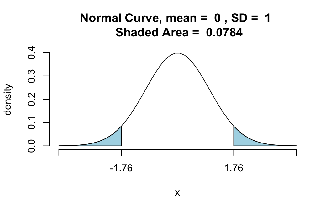
Anytime you want, you can get a graph of the \(P\)-value for your test, simply by setting the argument graph to TRUE:
proptestGC(~sex,data=m111survey,p=0.50,
        success="female",graph=TRUE)
##
##
## Inferential Procedures for a Single Proportion p:
## Variable under study is sex
## Continuity Correction Applied to Test Statistic
##
##
## Descriptive Results:
##
## female n estimated.prop
## 40 71 0.5634
##
##
## Inferential Results:
##
## Estimate of p: 0.5634
## SE(p.hat): 0.05886
##
## 95% Confidence Interval for p:
##
## lower.bound upper.bound
## 0.448016 0.678745
##
## Test of Significance:
##
## H_0: p = 0.5
## H_a: p != 0.5
##
## Test Statistic: z = 0.9571
## P-value: P = 0.3385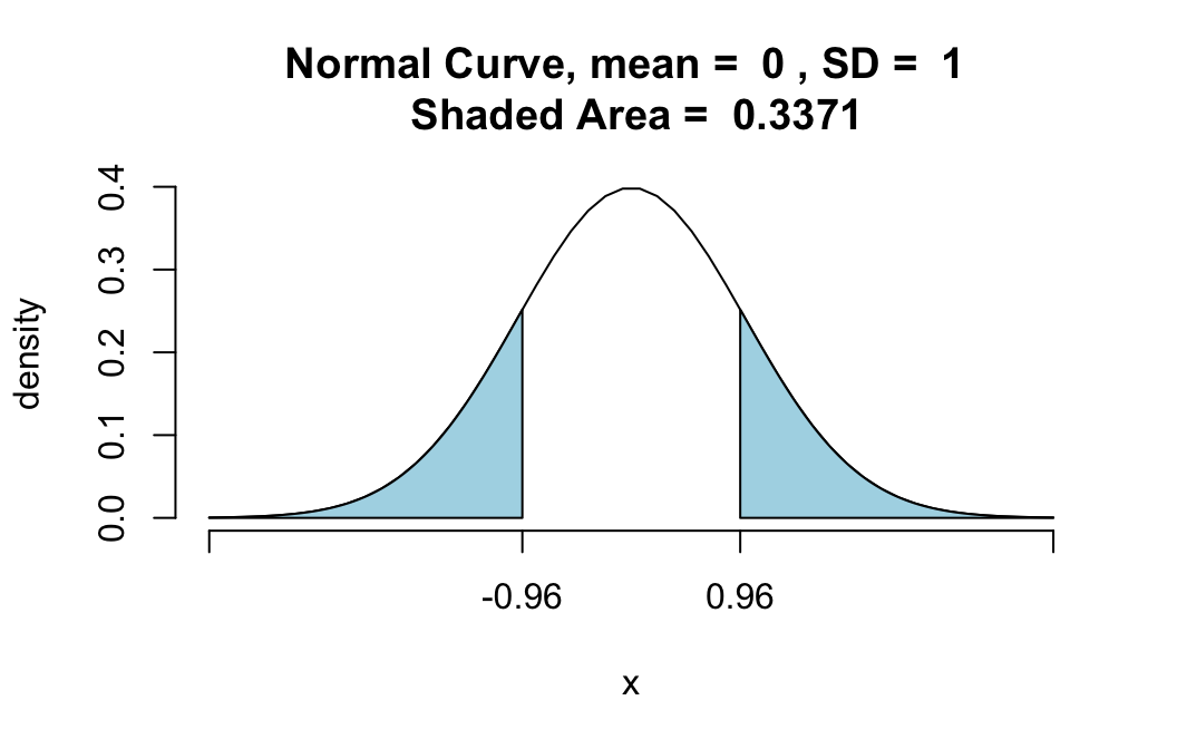
Limiting Output
Sometimes you don’t need R to print so much information to the console. If you want only the basics (such as a confidence interval, the test statistic and \(P\)-value), then set the verbose argument to FALSE:
proptestGC(~sex,data=m111survey,p=0.50,
        success="female",verbose=FALSE)
##
##
## Inferential Procedures for a Single Proportion p:
## Variable under study is sex
## Continuity Correction Applied to Test Statistic
## 95% Confidence Interval for p:
##
## lower.bound upper.bound
## 0.448016 0.678745
##
## Test Statistic: z = 0.9571
## P-value: P = 0.3385One Proportion, From Summary Data
Again note that binomtestGC() is preferred in this situation, especially at smaller sample sizes.
Confidence Interval Only
Say that you have taken a simple random sample of size \(n=2500\) from the population of all registered voters in the U.S., and you find that 1325 of them favor the Affordable Care Act. Suppose that you would like to make a confidence interval for
\(p =\) the proportion of all registered voters in the U.S. who support the Act.
You don’t have the raw data present in a data frame, but you have enough summary data to use proptestGC(). You just have to set some new arguments:
- set
xto 1325, the number of “successes” you are counting up; - set
nto 2500, the sample size.
So if you only want a 95%-confidence interval for \(p\). use:
proptestGC(x=1325,n=2500)##
##
## Inferential Procedures for a Single Proportion p:
## Results based on Summary Data
## Continuity Correction Applied to Test Statistic
##
##
## Descriptive Results:
##
## successes n estimated.prop
## 1325 2500 0.53
##
##
## Inferential Results:
##
## Estimate of p: 0.53
## SE(p.hat): 0.009982
##
## 95% Confidence Interval for p:
##
## lower.bound upper.bound
## 0.510436 0.549564Interval and Test
If you also want to do a test of significance, again specify p and alternative. For example, to test the hypotheses
\(H_0: p = 0.50\)
\(H_a: p < 0.50\)
use:
proptestGC(x=1325,n=2500,
        p=0.50,,alternative="less")
##
##
## Inferential Procedures for a Single Proportion p:
## Results based on Summary Data
## Continuity Correction Applied to Test Statistic
##
##
## Descriptive Results:
##
## successes n estimated.prop
## 1325 2500 0.53
##
##
## Inferential Results:
##
## Estimate of p: 0.53
## SE(p.hat): 0.009982
##
## 95% Confidence Interval for p:
##
## lower.bound upper.bound
## 0.000000 0.546419
##
## Test of Significance:
##
## H_0: p = 0.5
## H_a: p < 0.5
##
## Test Statistic: z = 3.025
## P-value: P = 0.9988Difference of Two Proportions, Data Frame
Confidence Interval Only
Suppose
\(p_1 =\) proportion of all GC females who believe they get enough sleep
\(p_2 =\) proportion of all GC males who believe they get enough sleep
If you desire, say, an 85%-confidence interval for \(p_1 - p_2\), then use:
proptestGC(~sex+enough_Sleep,data=m111survey,
        success="yes",conf.level=0.85)
##
##
## Inferential Procedures for the Difference of Two Proportions p1-p2:
## enough_Sleep grouped by sex
##
##
## Descriptive Results:
##
## yes n estimated.prop
## female 14 40 0.3500
## male 11 31 0.3548
##
##
## Inferential Results:
##
## Estimate of p1-p2: -0.004839
## SE(p1.hat - p2.hat): 0.1143
##
## 85% Confidence Interval for p1-p2:
##
## lower.bound upper.bound
## -0.169426 0.159749Interval and Test
If you want a 95%-confidence interval for \(p\_1 - p_2\) and you would like to test the hypotheses:
\(H_0: p_1 - p_2 = 0\)
\(H_a: p_1 - p_2 \neq 0\)
then use:
proptestGC(~sex+enough_Sleep,data=m111survey,
      success="yes",p=0)
##
##
## Inferential Procedures for the Difference of Two Proportions p1-p2:
## enough_Sleep grouped by sex
##
##
## Descriptive Results:
##
## yes n estimated.prop
## female 14 40 0.3500
## male 11 31 0.3548
##
##
## Inferential Results:
##
## Estimate of p1-p2: -0.004839
## SE(p1.hat - p2.hat): 0.1143
##
## 95% Confidence Interval for p1-p2:
##
## lower.bound upper.bound
## -0.228929 0.219252
##
## Test of Significance:
##
## H_0: p1-p2 = 0
## H_a: p1-p2 != 0
##
## Test Statistic: z = -0.04232
## P-value: P = 0.9662Notice that this time:
- you specified the Null’s belief about the value of \(p\_1-p_2\) using the
pargument; - you did not have to set
conf.levelto 0.95 (the default value of the argument is 0.95 already); - you did not have to specify the two-sided alternative (the default value of
alternativeis already “two.sided”).
Order of the Groups
Suppose that in the previous situation you had defined:
\(p_1 =\) proportion of all GC males who believe they get enough sleep
\(p_2 =\) proportion of all GC females who believe they get enough sleep
Then for you, the first population is all GC males and the second population is all GC females. In order to guarantee that R abides by your choice, use the argument first:
proptestGC(~sex+enough_Sleep,data=m111survey,
      success="yes",p=0,first="male")
##
##
## Inferential Procedures for the Difference of Two Proportions p1-p2:
## enough_Sleep grouped by sex
##
##
## Descriptive Results:
##
## yes n estimated.prop
## male 11 31 0.3548
## female 14 40 0.3500
##
##
## Inferential Results:
##
## Estimate of p1-p2: 0.004839
## SE(p1.hat - p2.hat): 0.1143
##
## 95% Confidence Interval for p1-p2:
##
## lower.bound upper.bound
## -0.219252 0.228929
##
## Test of Significance:
##
## H_0: p1-p2 = 0
## H_a: p1-p2 != 0
##
## Test Statistic: z = 0.04232
## P-value: P = 0.9662Difference of Two Proportions, Summary Data
Confidence Interval Only
Suppose that you have taken two independent samples from two populations (or performed a completely randomized experiment with two treatment groups), and you have the following summary data:
| Group | Success Count | Sample Size |
|---|---|---|
| group one | 1325 | 2500 |
| group two | 905 | 1800 |
You need to provide the summary data to the arguments x and n as lists using the c() function. In each list, data from the first group should come first.
For a 95%-confidence interval for \(p_1 - p_2\), use:
proptestGC(x=c(1325,905),n=c(2500,1800))##
##
## Inferential Procedures for the Difference of Two Proportions p1-p2:
## Results taken from summary data.
##
##
## Descriptive Results:
##
## successes n estimated.prop
## Group 1 1325 2500 0.5300
## Group 2 905 1800 0.5028
##
##
## Inferential Results:
##
## Estimate of p1-p2: 0.02722
## SE(p1.hat - p2.hat): 0.01544
##
## 95% Confidence Interval for p1-p2:
##
## lower.bound upper.bound
## -0.003048 0.057492Interval and Test
Suppose that you want a 90%-confidence interval for \(p_1 - p_2\) and that you would like to test the hypotheses:
\(H_0: p_1 - p_2 = 0\)
\(H_a: p_1 - p_2 > 0\)
Suppose also that you want a graph of the \(P\)-value. Then use:
proptestGC(x=c(1325,905),n=c(2500,1800),
           p=0,conf.level=0.90,graph=TRUE)
##
##
## Inferential Procedures for the Difference of Two Proportions p1-p2:
## Results taken from summary data.
##
##
## Descriptive Results:
##
## successes n estimated.prop
## Group 1 1325 2500 0.5300
## Group 2 905 1800 0.5028
##
##
## Inferential Results:
##
## Estimate of p1-p2: 0.02722
## SE(p1.hat - p2.hat): 0.01544
##
## 90% Confidence Interval for p1-p2:
##
## lower.bound upper.bound
## 0.001819 0.052626
##
## Test of Significance:
##
## H_0: p1-p2 = 0
## H_a: p1-p2 != 0
##
## Test Statistic: z = 1.763
## P-value: P = 0.07797