16 Recursion

Figure 16.1: The Sierpinski Triangle.

16.1 What is Recursion? Some Basic Examples

16.1.1 Example: Counting Down

Imagine that you are going to shoot off a toy rocket. To increase the dram for you and your friends, you will count down:

“5, 4, 3, 2, 1, Blastoff!”

You could count down from any number \(n\) that is at least 0. (Counting down from 0 means saying only “Blastoff!”):

\(n,\,n-1,\,n-2,\, \ldots,\, 2,\, 1,\, \text{Blastoff!}\)

If we want to write a function to count down from any non-negative integer \(n\), we could use a loop:

countdown_loop <- function(n) {
  while (n > 0) {
    cat(n, ", ...\n", sep = "")
    n <- n - 1
  }
  cat("Blastoff!")
}

Let’s watch it in action:

countdown_loop(n = 5)

## 5, ...
## 4, ...
## 3, ...
## 2, ...
## 1, ...
## Blastoff!

Perfectly fine!

But there is another way to look at the situation. Notice that when you finish saying “5, …”, what remains is to count down from 4, and in general, when you say your first number \(n\) what remains is to count down from \(n-1\).

Thus countdowns have what we call a recursive structure: any countdown contains within itself another, smaller countdown. The very smallest countdown is “Blastoff”, the countdown from 0.

In fact one could give “recursive” directions for performing countdowns as follows:

To perform the countdown from 0, say “Blastoff!”
For any integer \(n \geq 1\), to perform the countdown from \(n\) you say the number \(n\) and then perform the countdown from \(n-1\).

The first rule above is called the base case. At the base case, you know exactly what to do: just say “Blastoff”.

for higher values of \(n\), \(n=4\), say, you don’t know everything about what you need to do. But:

the second rule, which is called the recursive case, can be applied: it tells you to say “4”, and then to perform a countdown from 3.
To figure out how to count down from 3, you again apply the recursive case, saying “3”, and then you must figure out how to count down from 2.
The recursive rule applies again, telling you to say “2” and then count down from 1.
To count down from 1, the recursive rule applies once more, telling you to say “1” and then count down from 0.
Finally, the base case kicks in: counting down from 0 is done by just saying “Blastoff!”.

We can implement this recursive procedure in a function as follows:

countdown <- function(n) {
  ## Base case:
  if (n == 0) return(cat("Blastoff!"))
  ## Recursive case:
  cat(n, ", ...\n", sep = "")
  Recall(n - 1)
}

In the code above, the term Recall is a placeholder for the name of the function that has been called and whose runtime we are in. Thus it makes a call to coutndown().

Let’s try it out:

countdown(5)

## 5, ...
## 4, ...
## 3, ...
## 2, ...
## 1, ...
## Blastoff!

It works!

When the body of a function includes a call to the function itself, we say that the function is recursive. countdown() is a recursive function.

16.1.2 Example: Handshakes

We would like to write a function that solves the following problem:

\(n\) people are in a room. Each person shakes the hand of each other person. How many handshakes are there?

One way to approach the problem is to observe that the all-around handshakes have a recursive structure:

Base Case: When there is only one person involved no hands need to be shaken, so the number of handshakes is 0.
Recursive Case: For any integer \(n > 1\), if there are \(n\) people involved, then pick out one person and have that person shake hands with each of the other \(n-1\) people. That’s \(n-1\) handshakes. Then make that person leave the room, and have the remaining \(n-1\) people shake hands.

If we think of this in terms of a function called handshakes(), then the above two rules can be stated as follows:

Base Case: handshakes(1) = 0.
Recursive Case: for any \(n > 1\), handshakes(n) = n - 1 + handshakes(n-1).

We can implement this thinking in a recursive function:

handshakes <- function(n) {
  ## Base case:
  if (n == 1) {
    return(0)
  }
  ## Recursive case:
  n - 1 + Recall(n - 1)
}

Let’s try it out:

handshakes(4)

## [1] 6

16.1.3 Example: Fibonacci Sequence

The Fibonacci numbers are defined as follows:

\(F_1 = 1\)
\(F_2 = 1\)
For all \(n \geq 3\), \(F_n = F_{n-1} + F_{n-2}\)

Can we write a function to compute the \(n\)-th Fibonacci number, for any \(n \geq 1\)?

Indeed we can:

fib <- function(n) {
  ## Base cases:
  if (n %in% c(1, 2)) {
    return(1)
  }
  ## Recursive case:
  Recall(n - 1) + Recall(n - 2)
}

Let’s try it out:

fib(9)

## [1] 34

For reference, here are the first ten Fibonacci numbers:

`n`	`fib(n)`
1	1
2	1
3	2
4	3
5	5
6	8
7	13
8	21
9	34
10	55

16.1.4 Example: Conversion to a Given Base

in a previous chapter we looked at the problem of expressing a given positive integer in any given base-system. We came up with this function:

## b is the base, n is the number to express
to_base_loop <- function(b, n) {
  if (b > 36) stop("choose a lower base")
  digits <- c(0:9, letters)[1:b]
  numeral <- ""
  curr <- n
  while (curr >= b) {
    quot <- curr %/% b
    rem <- curr %% b
    numeral <- str_c(digits[rem + 1], numeral, sep = "")
    curr <- quot
  }
  str_c(digits[curr + 1], numeral, sep = "")
}

to_base(7, 5463)

## [1] "21633"

The function used a loop. However, we can also think of the problem recursively.

Consider, for example, the issue of expressing the number 43 in base 5. when we begin, we wonder what the “ones-place” should be, so we divide 43 by getting, getting a quotient of 8 and and a remainder of 3. now we know that the ones place should be 3.

Next, the quotient of 8 tells us that there are 8 fives left to express. We know that this works out to one 25 and three fives, so that:

\[43 = 1 \times 5^2 + 3 \times 5^1 + 3 \times 5^0,\] meaning that the base-five representation of 43 is 133.

But take a look at the initial “13” in the expression “133”. Standing by itself, 13 would be the base-five representation of the number 8, the quotient that we found!

So it seems that we can write a two-part rule for finding the base-five representation of any non-negative integer \(n\):

Base Case:
- if \(n = 0\), then the base-five representation is 0;
- if \(n = 1\), then the base-five representation is 1;
- if \(n = 2\), then the base-five representation is 2;
- if \(n = 3\), then the base-five representation is 3;
- if \(n = 4\), then the base-five representation is 4.
Recursive Case: If \(n \geq 5\), then divide \(n\) by 5 to get a quotient \(q\) and a remainder \(r\). The base-five representation of \(n\) is the base-five representation of \(q\) followed by the digit for \(r\).

We can express our thinking in a recursive function (generalized here to more bases):

to_base_rec <- function(b, n) {
  if (b > 36) stop("choose a lower base")
  digits <- c(0:9, letters)[1:b]
  ## base case
  if (n < b) return(digits[n + 1])
  ## recursive case:
  quot <- n %/% b
  rem <- n %% b
  str_c(Recall(b, quot), digits[rem + 1], sep = "")
}

Let’s try it out:

to_base_rec(5, 43)

## [1] "133"

Indeed, it works!

In general, any function that can be computed with iteration can also be written recursively, and vice-versa. Sometimes it’s easier to think in terms of iteration, and other times in terms of recursion.

16.1.5 Possible Problem: Lots of Re-Calls!

Look back at our recursive fib() function. For small values of \(n\), fib(n) runs quickly:

fib <- function(n) {
  ## Base cases:
  if (n %in% c(1, 2)) {
    return(1)
  }
  ## Recursive case:
  Recall(n - 1) + Recall(n - 2)
}

fib(6)

## [1] 8

But try this on your own:

fib(30)

it takes a scarily long time to finish! Don’t even bother with:

fib(50)

Why is the running time so long? Well, consider the following diagram of the function calls involved in a call to fib(6):

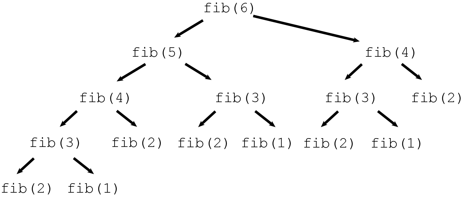
Figure 16.2: Function calls to determine the 6th Fibonacci number recursively. (Image credit: https://willrosenbaum.com

You see that until you get down to a base case (\(n=1\) or \(n=2\)), you have to do two recalls, so the tree of calls gets big quickly as \(n\) increases.

We can keep track of the number of calls, if we like:

counter <- 0
fib2 <- function(n) {
  counter <<- counter + 1
  if (n %in% c(1, 2)) {
    return(1)
  }
  Recall(n - 1) + Recall(n - 2)
}
fib2(10)

## [1] 55

counter

## [1] 109

Math Fact: the number of calls made by the fib() function when finding the nth Fibonacci number is \(2 \times F_n - 1.\)

This fact can be proved using mathematical induction, a proof technique that will be familiar to students who have taken a course in discrete mathematics. If you don’t know about mathematical induction but still want some evidence that the math statement is true, consider the following investigation via code:

## highest fib number to find:
m <- 25
## set up some results vectors:
calls <- numeric(m)
fibs <- numeric(m)
for (i in 1:m) {
  counter <- 0
  fibs[i] <- fib2(i)
  calls[i] <- counter
}

calls - (fibs + fibs - 1)

##  [1] 0 0 0 0 0 0 0 0 0 0 0 0 0 0 0 0 0 0 0 0 0 0 0 0 0

This verifies the math statement for the first 25 Fibonacci numbers.

It won’t do to have recursion work so slowly, so in a later section we’ll consider a way to speed things up.

16.2 Application: Weighted Directed Acyclic Graphs

In this section we will apply the idea of recursive functions to solve problems involving graphs. Graphs are mathematical structures that have many practical applications.

16.2.1 Definition and Examples

We will begin with two undefined terms: node and edge. You can think of a node as a circle or a dot. You can think of an edge as a line that connects one node to another node.

A graph is a set of nodes, with edges between some of them.

Not every node has to be connected to other nodes. A node in a graph that is not connected to any other node in the graph is called an isolated node.

A directed graph is a set of nodes with arrows between some of them.

A path in a directed graph is a sequence of nodes, where each node is connected to the next node by an arrow. for example:

\(n_1 \rightarrow n_2 \rightarrow \ldots \rightarrow n_m\)

Note that in a path, all of the arrows “go in the same direction”. So the following:

\(n_1 \rightarrow n_2 \leftarrow n_3\)

does not count as a path.

A cycle is a path that begins and ends at the same node.

A directed acyclic graph is a directed graph that has no cycles.

Note: Sometimes DAGS are called trees, but in the mathematics of graph theory a tree is a slightly different thing.

If there is an arrow from node \(a\) to node \(b\):

\(a \rightarrow b\)

then \(b\) is said to be a child of \(a\) and \(a\) is said to be a parent of \(b\).

If there is a path from node \(a\) to node \(b\), then \(b\) is said to be a descendant of \(a\), and \(a\) is said to be an ancestor of \(b\).

In a directed graph, a root node is a node that has no parents. A leaf node is a node that has no children.

Note: In our work with DAGs, we will assume that the DAG has finitely many nodes, and that there is exactly one root node.

A weighted graph is a graph where each node is assigned a numerical value, called its weight.

Our aim in this section is to solve problems involving weighted directed acyclic graphs (WDAGs).

Here is an example of a WDAG:

In the above WDAG, focus on any node you like, and consider that node together with all of its descendants, including the arrows between them. Perhaps you might focus on the node labeled “a” that has the weight 3. That node plus all its descendants looks like this:

That subgraph is itself a DAG! This always happens: the sub-graph of a DAG that is formed by a node and its descendants is itself a DAG.

If you chose the root node to focus on, then you got the original WDAG, but if you chose any other node then you got a smaller WDAG. The smallest WDAGS are the ones you get by focusing on a leaf-node: then the WDAG consists of that node alone.

Since in this way the parts of a DAG are themselves DAGS, DAGS are said to have a “recursive” structure. In fact, an alternative way to define a DAG is to do so “recursively”, as follows:

A single node without arrows counts as a DAG.

If \(G_1, G_2, \ldots, G_n\) are DAGS having root nodes \(r_1, r_2, \ldots, r_n\) respectively and if you introduce a new node \(R\) and make arrows from \(R\) to each of the nodes \(r_1, r_2, \ldots, r_n\), then the resulting structure counts as a DAG.

Accordingly, you can readily determine many features of a DAG (or a WDAG) using recursive functions.

If you like, you can make your own WDAGS. Attach the following two packages:

library(bcscr)
library(DiagrammeR)

The function make_val_tree() from the bcscr package makes WDAGS with a bit of randomness to them. Here is an example:

tr <- make_val_tree(
  min_children = 1,
  max_children = 3,
  min_depth = 3,
  values = -2:5,
  seed = 4949
)

There are a couple of ways to examine the WDAG tr. You could just look at a print-out in the console:

tr

##                levelName
## 1  R: 5                 
## 2   °--a: -2            
## 3       ¦--a: 3         
## 4       ¦   ¦--a: 2     
## 5       ¦   ¦   ¦--a: -2
## 6       ¦   ¦   °--b: 1 
## 7       ¦   ¦--b: 4     
## 8       ¦   °--c: -1    
## 9       °--b: 4         
## 10          °--a: 2

Alternatively, you can plot tr:

plot(tr)

Each node in a WDAG made by the make_val_tree() function has two properties:

value: the numerical value associated with the node;
children: a list of the nodes that are its children (this is NULL if the node is a leaf).

For example, to get the children of the root node, just run:

tr$children

## $`a: -2`
##           levelName
## 1 a: -2            
## 2  ¦--a: 3         
## 3  ¦   ¦--a: 2     
## 4  ¦   ¦   ¦--a: -2
## 5  ¦   ¦   °--b: 1 
## 6  ¦   ¦--b: 4     
## 7  ¦   °--c: -1    
## 8  °--b: 4         
## 9      °--a: 2

To get the children of the first child of the root node, just run:

tr$children[[1]]$children

## $`a: 3`
##       levelName
## 1 a: 3         
## 2  ¦--a: 2     
## 3  ¦   ¦--a: -2
## 4  ¦   °--b: 1 
## 5  ¦--b: 4     
## 6  °--c: -1    
## 
## $`b: 4`
##   levelName
## 1  b: 4    
## 2   °--a: 2

16.2.2 Recursive Functions for WDAGS

When you want to compute something recursively in a WDAG:

leaves will be base cases;
for other nodes, we make recursive calls on their children.

16.2.2.1 The Max-Weight Path Through a DAG

For example, consider the following question:

Given a WDAG, what path from the root node to a leaf has the maximum sum of weights?

Consider the WDAG below:

The weight of the maximum-weight path is \(5 + (-2) + 3 + 4 = 10.\)

In order to write a recursive function to solve find a path from root to a leaf that has the maximal weight, we consider:

A leaf would be a base case, because the only path from root to leaf is just the leaf itself, and of course the weight of that path is the value of the leaf.
For any WDAG that is not a leaf, consider the sub-graph WDAGs formed by each of the children of the root node. If we knew a maximal-weight path for each of these WDAGs, then we just take the sub-graph whose maximal-weight path is the smallest. Then we attach the root to this path and we have a path from root to leaf in the original WDAG whose weight it as small as possible.

The function below implements our thinking:

max_path <- function(node) {
  ## deal with base cases:
  if (is.null(node$children)) return(node$value)
  ## recursive cases:
  kids <- node$children
  path_values <- numeric(length = length(kids))
  for (i in 1:length(kids)) {
    path_values[i] <- Recall(kids[[i]])
  }
  return(node$value + max(path_values))
}

Let’s try it out:

max_path(node = tr)

## [1] 10

It works!

16.2.2.2 Max-Weight Sub-Trees

A sub-tree of a DAG is a node of the DAG together with all of its descendants. As we have seen, a sub-tree is also a WDAG.

Consider the following problem:

For any given WDAG, find a sub-tree whose total weight is as large as possible.

Again, let’s make a WDAG with which to work:

tr2 <- make_val_tree(
  min_children = 2,
  max_children = 2, 
  min_depth = 3,
  values = -8:10, seed = 5050
)

Below is a plot of tr2, with a maximal-weight sub-tree shown:

To write a recursive function to find the weight of a maximal sub-tree, we think as follows:

A leaf is a base case. (The leaf itself is its only sub-tree, so it is the sub-tree of maximal weight.)
If the WDAG is not a leaf, consider its root node, and suppose that we could find a maximal sub-tree for each of the WDAGs formed by its children. We can compare the weights of these maximal sub-trees with the weight of the entire WDAG, and pick the largest value.

From the above, it is clear that when we examine a WDAG, we have to find not only a maximal sub-tree and its weight, we must also compute the weight of the entire graph. Hence our recursive function should return two numbers: the weight of the entire graph and the weight of a maximal-weight sub-tree of the graph.

We implement our thinking as follows:

max_subtree <- function(node) {
  ## base cases:
  if (is.null(node$children)) {
    return(
      list(
        sum = node$value,
        m = node$value
      )
    )
  }
  ## recursive cases:
  kids <- node$children
  st_vals <- top_vals <- numeric(length = length(kids))
  for (i in 1:length(kids)) {
    res <- Recall(kids[[i]])
    st_vals[i] <- res$sum
    top_vals[i] <- res$m
  }
  return(
    list(
      sum = node$value + sum(st_vals),
      m = max(node$value + sum(st_vals), top_vals)
    )
  )
}

Let’s try it out:

max_subtree(tr2)

## $sum
## [1] 68
## 
## $m
## [1] 75

The weight of the entire WDAG is 68.
The weight of the maximal sub-tree is 75.

16.3 Interlude: Lexical Scoping in R

16.3.1 A Gift-Giving Clown

Let’s write a function to simulate a clown that has a bag of prizes. whenever the function is run, the clown should pick a prize at random from its bag and give it away.

clown <- function() {
  bag <- c("mustang", "goat", "20 dollar bill")
  cat("Hello, my name is Alfie!\n")
  if (length(bag) == 0) {
    sad_message <-"Sorry, the bag is empty!"
    return(cat(sad_message))
  }
  gift_number <- sample(1:length(bag), size = 1)
  gift <- bag[gift_number]
  cat("Here, have a ", gift, "!", sep = "")
  cat("\n\n")
  # clown removes gift from bag:
  bag <- bag[-gift_number]
}

Now let’s have the clown go around town, giving gifts:

clown()

## Hello, my name is Alfie!
## Here, have a mustang!

clown()

## Hello, my name is Alfie!
## Here, have a 20 dollar bill!

clown()

## Hello, my name is Alfie!
## Here, have a mustang!

clown()

## Hello, my name is Alfie!
## Here, have a goat!

Clearly there is an issue here! the clown should have run out of gifts after the first three function calls.

The problem is that every time clown() is run, bag is set to the vector of three items: the mustang, the goat, and the 20-dollar bill.

This means that following line in the body of the function:

bag <- bag[-gift_number]

was completely useless!

There is a simple workaround, involving the so-called “super-assignment” operator <<-.

We consult the help on <<-:

help("<<-")

We read that <<- causes:

“a search to be made through parent environments for an existing definition of the variable being assigned. If such a variable is found (and its binding is not locked) then its value is redefined, otherwise assignment takes place in the global environment.”

This inspires us to write a new version of the clown function:

## the bag is defined in the Global Environment:
bag <- c("mustang", "goat", "20 dollar bill")

## the new clown-giving function
clown <- function() {
  cat("Hello, my name is Alfie!\n")
  if (length(bag) == 0) {
    sad_message <-"Sorry, the bag is empty!"
    return(cat(sad_message))
  }
  gift_number <- sample(1:length(bag), size = 1)
  gift <- bag[gift_number]
  cat("Here, have a ", gift, "!", sep = "")
  cat("\n\n")
  ## use the super-assignment operator to change bag
  bag <<- bag[-gift_number]
}

Let’s try out the new clown function:

clown()

## Hello, my name is Alfie!
## Here, have a mustang!

clown()

## Hello, my name is Alfie!
## Here, have a 20 dollar bill!

clown()

## Hello, my name is Alfie!
## Here, have a goat!

clown()

## Hello, my name is Alfie!
## Sorry, the bag is empty!

It seems to be working fine: the clown gave out a different gift each time, running out after three function-calls.

However:

It’s dangerous to have a function messing with items in other environments. (What if you had some other use for an object named bag?)
If you want to have more than one clown going about town giving gifts, you would have to have a differently-named bag for each of them.

16.3.2 Lexical Scoping and Clown-Factories

Let’s make use of the following important rule in R:

In R, the parent environment of the runtime environment of a function is the environment in which the function was defined.

This is an instance of what is known in computer programming lexical scoping.

Here is an example of lexical scoping at work:

y <- 10
f <- function(x) {
  x + y
}
f(15)

## [1] 25

g <- function(x) {
  y <- 5
  f(x)
}
g(15)

## [1] 25

Observe that:

g(15) was NOT \(15 + 5 = 20\);
instead, g(15) was \(15 + 10 = 25\)

That’s because the parent environment of f() is the Global Environment (where f() was defined).

The parent environment of f() was NOT the run-time environment of g(). That was just an environment in which F() was called.

We can apply the idea of lexical scoping to solve the problem of where to store bags for clowns. We write a new function that returns clown-functions:

## a function to make clowns
clown_factory <- function(name, bag = c("million dollars", "new car")) {
  clown <- function() {
    cat("Hello, my name is ", name, "!\n", sep = "")
    if (length(bag) == 0) {
      sad_message <-"Sorry, the bag is empty!"
      return(cat(sad_message))
    }
    gift_number <- sample(1:length(bag), size = 1)
    gift <- bag[gift_number]
    cat("Here, have a ", gift, "!\n", sep = "")
    cat("\n\n")
    ## use the super-assignment operator to change bag
    bag <<- bag[-gift_number]
  }
  ## now return this clown-function:
  clown
}

Now let’s make a few clowns:

## clowns will issued bags like this:
bag <- c("mustang", "goat", "20 dollar bill")
## make three clowns:
alfie <- clown_factory(name = "Alfie", bag = bag)
bozo <- clown_factory(name = "Bozo")
chester <- clown_factory(name = "Chester",bag = bag)

Now let’s have the clowns go about town, giving gifts:

alfie()

## Hello, my name is Alfie!
## Here, have a goat!

alfie()

## Hello, my name is Alfie!
## Here, have a 20 dollar bill!

alfie()

## Hello, my name is Alfie!
## Here, have a mustang!

alfie()

## Hello, my name is Alfie!
## Sorry, the bag is empty!

bozo()

## Hello, my name is Bozo!
## Here, have a million dollars!

chester()

## Hello, my name is Chester!
## Here, have a goat!

Note that Alfie’s gift-giving did nothing to deplete the bags of Bozo or Chester.

None of these bags has anything to do with the bag that was defined in the Global Environment. In particular, that bag is unchanged:

bag

## [1] "mustang"        "goat"           "20 dollar bill"

Why does this work? Well, for each clown, its bag is in the run-time environment where the clown was defined. (That’s three different run-time environments!). Each clown searches its parent environment for bag when its function is called, and each clown finds a bag in its (own) parent environment.

16.4 Application: Recursion with Memoization

Let’s apply the idea of lexical scoping to make a recursive function run faster.

Consider the problem of finding Fibonacci numbers. When we have to generate Fibonacci numbers by hand, we don’t start from scratch with each new number. Instead, we think:

fib(1) is 1, by definition.
fib(2) is 1, by definition.
By definition fib(3) is fib(2) plus fib(1), and we know both of these are 1, so fib(3) is \(1+1=2\).
By definition fib(4) is fib(3) plus fib(2), and we already found that fib(3) is 2 and we know that fib(2) is 1, so fib(4) is \(2+1=3\).
and so on …

When we need the next Fibonacci number, we just “look up” the two previous Fibonacci numbers and add them.

The following function returns a function that will compute Fibonacci numbers. The body of the function defines a look-up table, called a memo sheet that can be augmented via super-assignment.

fib_mem_factory <- function(verbose = FALSE) {
  ## the memo sheet:
  known_fibs <- numeric()
  ## for verbose option, to count calls of the fib-function:
  counter <- 0
  function(n) {
    counter <<- counter + 1
    if (verbose) cat("this is call ", counter, "\n", sep = "")
    if (n <= length(known_fibs) & !is.na(known_fibs[n])) {
      if (verbose) cat("we already know this one!\n")
      return(known_fibs[n])
    }
    if (n %in% c(1, 2)) {
      if (verbose) cat("got to a base fib-value\n")
      known_fibs[n] <<- 1
      return(1)
    }
    if (verbose) cat("finding fib", n-2, "\n")
    fibp <- Recall(n - 2)
    if (verbose) cat("finding fib ", n-1, "\n")
    fibpp <- Recall(n - 1)
    new_fib <- fibp + fibpp
    known_fibs[n] <<- new_fib
    new_fib
  }
}

Let us now make a function to compute Fibonacci numbers:

fib_better <- fib_mem_factory(verbose = FALSE)

Let’s try it out:

fib_better(30)

## [1] 832040

fib_better(50)

## [1] 12586269025

This function works ever so much faster than the old fib()!

If we use the verbose option, we can understand why this is true:

fib_better_2 <- fib_mem_factory(verbose = TRUE)
fib_better_2(n = 5)

## this is call 1
## finding fib 3 
## this is call 2
## finding fib 1 
## this is call 3
## got to a base fib-value
## finding fib  2 
## this is call 4
## got to a base fib-value
## finding fib  4 
## this is call 5
## finding fib 2 
## this is call 6
## we already know this one!
## finding fib  3 
## this is call 7
## we already know this one!

## [1] 5

Because we use the memo sheet so much, we need far fewer recalls.

Links to Slides

Quarto Presentations that I sometimes use in class:

Glossary

Recursive Function: A function that calls itself somewhere in its own body.
Base Case: In a recursive function, the input(s) for which the function will return a value without having to recall itself.
Recursive Case: In a recursive function, the input(s) for which the function must recall itself in order to compute the value it will return.
Graph: A set of nodes, with edges between some of them.
Directed Graph: A set of nodes with arrows between some of them.
Path: A sequence of nodes in a directed graph, where each node is connected to the next node by an arrow, with all arrows pointing the same way.
Cycle: A path that begins and ends at the same node.
Directed Acyclic Graph (DAG): A directed graph that has no cycles.
Weighted Directed Acyclic Graph: A directed acyclic graph where each node is assigned a number, called its weight.
Parent/Child: In a directed graph, if there is an arrow from node \(a\) to node \(b\) then \(b\) is said to be a child of \(a\) and \(a\) is said to be a parent of \(b\).
Ancestor/Descendant: In a directed graph, if there is a path from node \(a\) to node \(b\), then \(b\) is said to be a descendant of \(a\), and \(a\) is said to be an ancestor of \(b\).
Root: In a directed graph, a root node is a node that has no parents.
Leaf: In a directed graph, a leaf node is a node that has no children.

Exercises

Write a recursive function called is_palindrome() that, when given any vector, returns TRUE if the vector is the same as itself reversed, and returns FALSE otherwise. The function should take a single parameter called vec, the vector to check for being a palindrome.

Typical examples of use should be as follows:
```
## vectors of length 0 are palindromes:
is_palindrome(vec = character())
```
```
## [1] TRUE
```
```
is_palindrome(vec = "x")
```
```
## [1] TRUE
```
```
is_palindrome(vec = c(2, 2))
```
```
## [1] TRUE
```
```
is_palindrome(vec = c("b", "a", "b", "a"))
```
```
## [1] FALSE
```

Write a recursive function called substrings() that, when given any non-empty string, returns a character vector of the substrings of that string. The function should take a single parameter called str, the strings for which the substrings are found.

A typical example of use would be as follows:

## convenience function to order the
## elements of a character vector:
strings_ordered <- function(strs) {
  data.frame(
    strings = strs
  ) %>% 
    mutate(num_char = str_length(strings)) %>% 
    arrange(num_char, strings) %>% 
    pull(strings)
}

"yowsa" %>% 
  substrings() %>% 
  strings_ordered()

##  [1] "a"     "o"     "s"     "w"     "y"     "ow"    "sa"    "ws"    "yo"   
## [10] "ows"   "wsa"   "yow"   "owsa"  "yows"  "yowsa"

Write a recursive function called countup() will count up from a starting number to a finishing number. The function should take two parameters:
- start: the number at which to begin;
- n: the number at which to finish.
Typical examples of use should be as follows:
```
countup(start = 7, n = 6)
```
```
## start should not exceed n
```
```
countup(start = 6, n = 6)
```
```
## 6, ...
## All done!
```
```
countup(start = 1, n = 5)
```
```
## 1, ...
## 2, ...
## 3, ...
## 4, ...
## 5, ...
## All done!
```
In a weighted directed acyclic graph (WDAG), let us define a maximal subpath to be a path that begins at the root node and has a sum of node-values that is as large as possible. (Note that such a path need not continue all the way to a leaf.)

For example. consider the following WDAG:
```
wdag <- make_val_tree(
  min_children = 1,
  max_children = 3,
  values = -5:5,
  min_depth = 3,
  seed = 5556
)
```
A maximal subpath for our WDAG is shown below (node fill for the path is burlywood):

Write a function called max_subpath() that, when given any WDAG, will return the sum of the weights of the nodes for its maximal subpath(s). The function should take a single parameter called node, whose value would be a WDAG as constructed using data.tree in class.

Here is what we get when we apply such a function to our example WDAG:

max_subpath(node = wdag)

## [1] 6

15 Object-Oriented Programming in R

References