Chapter 10 Tests of Significance
10.1 Introduction
Confidence intervals aim to answer the question:
Given the data at hand, within what range of values does the parameter of interest probably lie?
Now we will turn to another important type of question in statistical inference:
Based on the data at hand, is it reasonable to believe that the parameter of interest is a particular given value?
When we address such a question, we perform a test of hypothesis (also called a test of significance).
In this Chapter we will look at significance tests for each of the Basic Five parameters, one by one. Although the parameters will vary from one research question to another, a test of hypothesis always follows the standard five-step format we studied back in Chapter 4. In what follows, we will go through each of the Basic Five parameters one by one. Our procedure will be as follows:
- State a Research Question that turns out to involve the parameter of interest.
- Write out all five steps of the test, calling a “packaged” R-function, the output of which we will use to fill in some of the steps. These functions produce confidence intervals for the parameter in question, so you will have met them already in the previous chapter on confidence intervals.
- Look “under the hood” of the test just a bit, to see how the packaged function is getting the test statistic and the P-value. We may also introduce some concepts or terminology that apply to all tests of significance, or to all tests involving one of the Basic Five.
- We will try one or two other examples involving the same parameter.
After each parameter has been covered, we will discuss some general issues in hypothesis testing. These considerations will apply to all of the tests introduced in this chapter, as well as to the chi-square test from Chapter 4.
Finally, we will undertake a “Grand Review”, in which we practice moving from a Research Question to the proper inferential procedures to address that question.
10.2 One Population Mean
10.2.1 Introductory Research Question
Consider the following Research Question concerning the mat111survey data:
Does the data provide strong evidence that the mean fastest speed for all Georgetown College exceeds 100 mph?
10.2.2 The Five Steps
Clearly, the parameter of interest is a single population mean. Unlike the situation with the chi-square test, the debate is about the value of a parameter. Hence Step One should include a clear definition of the parameter of interest, followed by a statement of Null and Alternative Hypotheses that lay out views concerning the value of this parameter.
Step One: Definition of parameter and statement of hypotheses.
We define the parameter first. Let
\(\mu\) = the mean fastest driving speed of ALL Georgetown College students.
Now that we have defined the parameter of interest, we can state our hypotheses in terms of that parameter, using the symbol we have defined:
\(H_0\): \(\mu = 100.\)
\(H_a\): \(\mu > 100.\)
Step Two: Safety Check and Reporting the Value of the Test Statistic
Just as chisqtestGC() was the work-horse for the \(\chi^2\) test for relationship between two factor variables, so in this Chapter there is an R-function that does much of the computational work we need for tests involving population means. In this case the function is the very same one that produced confidence intervals for us, namely: ttestGC(). We simply need to provide a couple of extra arguments in order to alert it to our need for a test of significance:
ttestGC(~fastest,data=m111survey,mu=100,
         alternative="greater")
The mu argument specifies the so-called “Null value”—the value that the Null hypothesis asserts for the parameter \(\mu\). The alternative argument indicates the “direction” of the Alternative Hypothesis—in this case, the Alternative asserts that \(\mu\) is greater than 100.
When we run the code above, we get results that will help us through Steps Two through Four in a test of significance.
The first thing we will do is the “safety check”. For each of the Basic Five parameters, the test of significance is built upon the same mathematical ideas that are used in the construction of a confidence interval. Hence the conditions for reliability of the tests are the same as for those of confidence intervals. In this case, we ask that the sample be roughly normal in shape, or that the sample size be at least 30. Hence we pay attention to the “Descriptive Results” first:
## Descriptive Results:
##
##  variable  mean    sd  n
##   fastest 105.9 20.88 71
We see that the sample size was \(n=71\), quite large enough to trust the approximation-routines that R uses for inferential procedures involving a mean.
The other element of the safety check is to ask whether our sample is like a simple random sample from the population. As we have seen with the mat111survey data, this is a debatable point: the sample consists of all students in MAT 111 from a particular semester, so it’s not really a random sample. On the other hand, for a question like “fastest speed ever driven”, it might be equivalent to a random sample. At any rate, we don’t have much reason to believe that there is a relationship between one’s fastest driving speed and whether or not one enrolls in MAT 111.
So much for the safety check. Now let’s go for the test statistic.
The test statistic in this test is called t. From the ttestGC() output, we see:
## Test Statistic: t = 2.382Apparently the test statistic is \(t=2.382\).
Step Three: Statement and Interpretation of the P-value
Again we read, from the function output, that:
## P-value: P = 0.009974The \(p\)-value is about 0.01, or 1%.
In this test, the way to interpret the P-value is as follows:
P-value Interpretation: If the mean fastest speed of all GC students is 100 mph, then there is about a 1% chance that the test statistic will be at least as big as the test statistic that we actually got.
Step Four: Decision
As we see from the interpretation of the P-value, a low P-value makes the Null appear to be implausible. Since P < 0.05 for us, we reject the Null Hypothesis.
Step Five: Write a Conclusion
As in Chapter Three, this should be a complete sentence in nontechnical language that says how much evidence the data provided for the Alternative Hypothesis. Our conclusion this time is:
This data provides strong evidence that the mean fastest speed for all GC students is greater than 100 mph.
10.2.3 Under the Hood, and Further Ideas
10.2.3.1 t-Statistic Formula
The formula for the t-statistic is:
\[t = \frac{\bar{x}-\mu_0}{s/\sqrt{n}},\]
where:
- \(\bar{x}\) is the sample mean,
- \(\mu_0\) is what the Null hypothesis thinks that \(\mu\) is, and
- \(s/\sqrt{n}\) is the SE for \(\bar{x}\), the same standard error that we have met in previous chapters.
Remember that the EV of \(\bar{x}\) is just \(\mu\), the mean of the population from which the sample was drawn. The Null believes that \(\mu\) is \(\mu_0\), so the Null expects \(\bar{x}\) to be about \(\mu_0\), give or take some for chance error. The numerator in the formula, \(\bar{x}-\mu_0\), is often called the observed difference, because it gives the difference between the sample mean that was actually observed and what a believer in the Null would expect that sample mean to be.
The denominator of the t-statistic gives the SE for \(\bar{x}\), which means that is gives the amount by which \(\bar{x}\) is liable to differ from the mean of the population. So if the Null is right, then \(\bar{x}\) says about how big the observed difference is liable to be.
The t-statistic divided the observed difference by the standard error. Hence the t-statistic is comparing the observed difference with how big the difference should be, if the Null is right. Another way of putting it is:
The t-statistic tells us how many stnadard errors the sample mean is above or below the value that the Null expects.
Consider the test statistic in our first example:
\[t \sim 2.38.\]
If we had wanted to, we could have computed the t-statistic from other elements of the test output. Part of the output gives:
## Estimate of mu:   105.9
## SE(x.bar):    2.478
So the observed difference is
\[\bar{x}-\mu_0=105.9-100-5.9\]
miles per hour. Dividing this by the standard error 2.478, we get:
\[t=\frac{5.9}{2.478} \approx 2.38.\]
The results tell us that our sample mean was 2.38 SEs above the value (100 mph) that the Null was expecting it to be. A little bit of give-and-take—due to chance error in the sampling process—is understandable, but these results are more than two SEs above what the Null would expect. Even before we look at the P-value, a large t-statistic tells us that the Null Hypothesis is implausible!
A t-statistic functions analogously to the z-score that we met back in Chapter 2. Just as a z-score tells us how many SDs an individual is above or below the mean for its groups, so the t-statistic tells us how many SEs the estimator is above or below what the Null expects it to be.
10.2.3.2 How the P-value is Computed
The P-value in this test is supposed to be the probability – given that the Null Hypothesis is true—of getting a t-statistic at least as big as 2.38, the test statistic that we actually got. Therefore, in order to compute this probability we have to know something about the distribution of the test statistic when the Null is true (sometimes this is called the Null distribution of t).
The key to the null distribution of t lies in a new family of distributions called the t-family. There is one member of the t-family for each positive integer, and this positive integer is called the degrees of freedom of the distribution. The distributions are all continuous, so they all have density curves. The following app lets you explore them:
require(manipulate)
tExplore()
Over a hundred years ago, William Gossett, the person who discovered the t-statistic, was able to relate the t-statistic to the t-curves.
He found that if:
- you take a random sample of size \(n\), at least 2, and
- the population you sample from is normally distributed, and
- the Null Hypothesis is true
then
- the t-statistic has the same distribution as the t-curve whose degrees of freedom is one less than the sample size \(n\).
So to find the P-value for your test, we only have to find the area under a t-curve with 70 degrees of freedom (one less than our sample size of 71), past our t-value 2.3818. We can do this with the r-function ptGC():
ptGC(2.3818,region="above",df=70)## [1] 0.009975159The shaded area is the P-value!
If you would like to see a graph of the P-value along with the results of the t-test, then in the ttestGC() function, simply set the argument graph to TRUE:
ttestGC(~fastest,data=m111survey,mu=100,
         alternative="greater",graph=TRUE)
10.2.3.3 Importance of Safety Checks
According to the mathematics that Gosset worked out, the P-value given by R’s routine is exactly correct only when we have a taken a random sample from a population that is EXACTLY normal in shape. Of course this never occurs in practice.
However, the P-value given by the ttestGC() is approximately correct if the population from which the sample is drawn is approximately bell-shaped. We can’t examine the entire population, but we could look at a histogram or a boxplot of the sample to see if the sample is approximately bell-shaped. If a histogram or boxplot of the sample reveals not too much skewness and no terribly large outliers, we take it as evidence that the population is roughly bell-shaped, in which case the Null distribution of the test statistic has approximately a t-distribution and so R’s P-value is approximately correct.
In general, the larger the sample size, the better the t-curve approximation is, even if the underlying population is far from normal. As a rule of thumb: when the sample size is more than 30, we accept the approximation given by the ttestGC() function, even if a histogram of the sample shows skewness and/or outliers.
In order to judge the effect of using the t-curve to approximate P-values, try the app tSampler() on a skewed population:
require(manipulate)
tSampler(~income,data=imagpop)
Try first at a very small sample size, such as \(n=2\), building the density curve for the t-statistics. After you have had enough, compare the density curve for your t-statistics with the t-curve that would give the correct distribution of the t-statistic if the underlying population were normal. Try again for a larger sample size, such as \(n=30\).
10.2.3.4 Further Examples
10.2.3.4.1 A One-Sided “Less Than” Test
Consider the following:
Research Question: The mean GPA of all UK students is known to be 3.3. Does the
mat111surveydata provide strong evidence that the mean GPA of all GC students is lower than this?
Step One: Definition of parameter and statement of hypotheses.
Let
\(\mu\) = the mean GPA of all GC students.
Then our hypotheses are:
\(H_0\): \(\mu=3.3\)
\(H_a\): \(\mu < 3.3\)
Note: This time, the alternative involves a “less than” statement. Both the original example and this example are “one-sided” tests, but the “side” differs.
Step Two: Safety Check and Test Statistic.
Again we run the test to extract information needed for steps Two through Four:
ttestGC(~GPA,data=m111survey,
         mu=3.3,alternative="less")
For the safety check, let’s first see if we have more than 30 students in the sample (if we do, we don’t have to make a histogram or boxplot of the sample).
##  variable  mean     sd  n
##       GPA 3.195 0.5067 70
Only one student did not report a GPA. The sample size is 70, which is bigger than 30, so we are safe to proceed.
Next we get the test statistic:
## Test Statistic: t = -1.733The test statistic is -1.73, so our sample mean of 3.19 was 1.73 SEs below what the Null was expecting.
Step Three: Statement of the P-value
## P-value: P = 0.04382The P-value was 0.044. It’s important to interpret it:
Interpretation of the P-value: If the mean GPA of all GC students is the same as it is at UK, then there is only about a 4.4% chance of getting a test statistic less than or equal to the one we actually got.
Note: When the alternative hypothesis involves “less than” then the P-value is the chance of getting results less than what we actually got, rather than greater than what we got. The P-value appears as a shaded area in Figure [One-Sided Less-Than P-Value].
ptGC(-1.73,region="below",df=70,graph=T)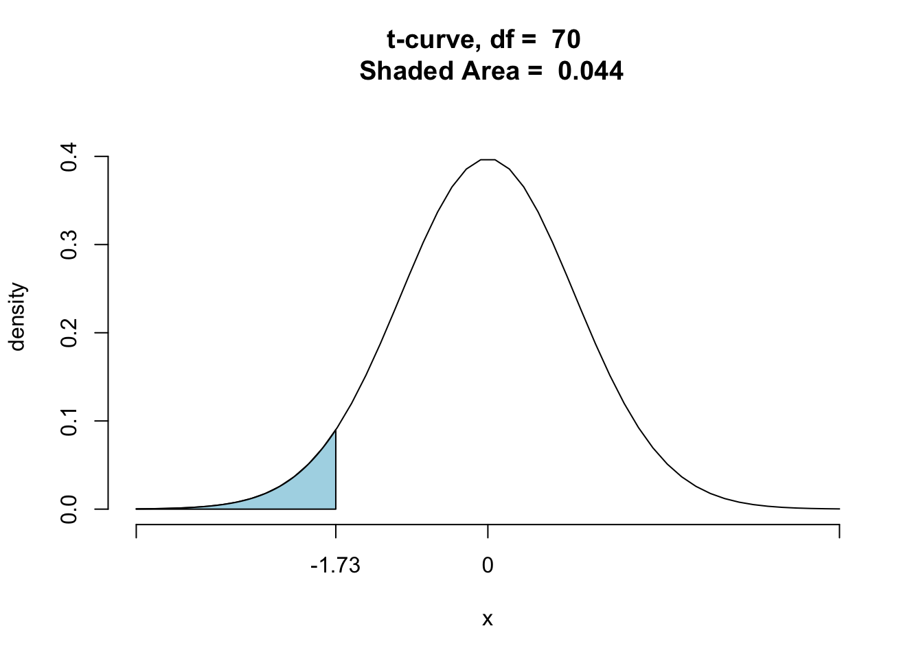
Figure 10.1: One-Sided Less-Than P-Value.
## [1] 0.04401866Step Four: Decision
Since the P-value was < 0.05, we reject the Null Hypothesis.
Step Five: Conclusion
This data provided strong evidence that the mean GPA at GC is less than it is at UK.
10.2.3.4.2 A Test From Summary Data
Sometimes you do not have access to the raw data in a data frame, and only summary statistics are available. You can still perform tests, if you are given sufficient summary information.
Suppose, for example, that the mean length of 16 randomly-caught Great White sharks is 14 feet, and that the standard deviation of the lengths is 3 feet. You are told that a histogram of the 16 weights looked fairly bell-shaped. You are asked to say whether the data provide strong evidence that the mean length of all Great Whites is less than 15 feet.
Step One: Definition of parameter and statement of hypotheses.
Let
\(\mu\) = the mean length of ALL Great White sharks.
Then our hypotheses are:
\(H_0\): \(\mu\) = 15
\(H_a\): \(\mu\) < 15
Step Two: Safety Check and Test Statistic
The sample size is 16 which is less than 30, but you are told that the sample is roughly normal. On that basis you hope that the population is roughly normal, so you decide that the P-value provided by ttestGC() is approximately correct.
The protocol for entering summary data is the same as it was for confidence intervals, except that you add the mu and alternative arguments:
ttestGC(mean=14,sd=3,n=16,,mu=15,alternative="less")##
##
## Inferential Procedures for One Mean mu:
##
##
## Descriptive Results:
##
## mean sd n
## 14 3 16
##
##
## Inferential Results:
##
## Estimate of mu: 14
## SE(x.bar): 0.75
##
## 95% Confidence Interval for mu:
##
## lower.bound upper.bound
## -Inf 15.314788
##
## Test of Significance:
##
## H_0: mu = 15
## H_a: mu < 15
##
## Test Statistic: t = -1.333
## Degrees of Freedom: 15
## P-value: P = 0.1012We see that the test statistic is t = -1.33
Step Three: P-value.
The P-value is 0.10.
Interpretation of P-value: If the mean length of all Great White sharks is 15 feet, then there is about a 10% chance of getting a t-statistic of -1.33 or less, as we got in our study.
Step Four: Decision
Since P > 0.05, we do not reject the Null Hypothesis.
Step Five: Conclusion
The data did not provide strong evidence that the mean length of all Great Whites is less than 15 feet.
10.3 Difference of Two Population Means
10.3.1 The Difference of Two Means
We will consider the following Research Question concerning the mat111survey data:
Research Question: Does the data provide strong evidence that GC males drive faster, on average, than GC females do?
10.3.2 The Five Steps
Step One: Define parameters and state hypotheses.
Although we are interested in only one number (the difference of two means) we have to define both population means in order to talk about that difference. Here we go:
Let
\(\mu_1\) = the mean fastest speed of all GC females.
\(\mu_2\) = the mean fastest speed of all GC males.
Now we can state the Hypotheses:
\(H_0\): \(\mu_1-\mu_2 = 0\)
\(H_a\): \(\mu_1-\mu_2 < 0\)
Step Two: Safety Check and Test Statistic.
As usual, we run the test in order to gather information needed for steps Two through Four:
ttestGC(fastest~sex,data=m111survey,mu=0,alternative="less")This time, the mu argument specifies the Null value of \(\mu_1-\mu_2\).
Just as with confidence intervals, the results of the packaged test that R performs are trustworthy only if the following are true:
- Either we took two independent random samples from two populations, or we did a completely randomized experiment and the two samples are the two treatment groups in that experiment
- Both populations are roughly normal, or else the sample sizes are both “large enough” (30 or more will do).
We’ll assume that the sample of males and the sample of females are like SRSs from their respective populations (at least as far as fastest speed is concerned),so Part 1 is OK. As for Part 2, it is doubtful that the two populations of fastest speeds are normal, but from the Descriptive Results (below) we see that our samples are indeed “big enough”:
##   group  mean    sd  n
##  female 100.7 17.82 38
##    male 113.9 22.81 30
Both sample sizes exceed 30. We squeaked by! If one of them had been less than 30 then we would have made a histogram of it and checked for strong skewness/outliers.
As for the test statistic, it is:
## Test Statistic: t = -2.725 We see that the value of the t-statistic is \(t = -2.735\).
Step Three: P-Value
From the output, we see that:
## P-value: P = 0.004289The P-value is about 0.0043, or 0.43%.
Interpretation of P-value: If males and females at GC drive equally fast on average, then there is only about a 0.43% chance of getting a t-statistic less than or equal to -2.735, as we did in our study.
Step Four: Decision about Null Hypothesis
Since P < 0.05, we reject \(H_0\).
Step Five: Conclusion
This data provided strong evidence that GC females drive slower than GC males do, on average.
10.3.3 Under the Hood
10.3.3.1 The Formula for the t-statistic
When we are testing the difference between two means, the formula for the t-statistic is:
\[t = \frac{\bar{x}_1-\bar{x}_2}{\sqrt{s_1^2/n_1+s_2^2/n_2}},\]
where:
- \(\bar{x}_1-\bar{x}_2\) is the difference between the sample means
- \(\sqrt{s_1^2/n_1+s_2^2/n_2}\) is the SE for the difference
Remember that if the Null is right, then \(\mu_1-\mu_2\) is 0, so the EV of \(\bar{x}_1-\bar{x}_2\) is 0. Hence the Null is expecting that the numerator of the t-statistic will work out to around 0, give or take a SE or two.
Therefore, just as in the case of one mean, the t-statistic compares the observed difference with the likely size of the observed difference, by dividing the former quantity by the latter.
This is a common pattern for the test statistics for Basic Five parameters:
\[\text{test statistic} = \frac{\text{observed difference}}{\text{SE for the difference}}.\]
Therefore when the test statistic is big, we know that the observed difference is many standard errors away from what the Null expects, and that looks bad for the Null Hypothesis.
10.3.3.2 Order of Groups
In the foregoing example, note that we have a one-sided “less than” alternative hypothesis, even though the research question asked if there was strong evidence that the mean speed of all GC males is GREATER than the mean speed of all GC females. This is because we have defined our first mean \(\mu_1\) as the mean speed of all females, so males being faster would imply that \(\mu_1-\mu_2\) is negative. R has certain defaults, usually involving alphabetical order, for which population to consider as the “first” one. If we wish to override these defaults we can do so, using the first argument:
ttestGC(fastest~sex,data=m111survey,
         mu=0,alternative="less",
         first="male")
10.3.3.3 The Degrees of Freedom in Two Samples
Look at the stated Degrees of Freedom in the output for our test:
## Degrees of Freedom: 55.49 It is not a whole number, nor it does not have any clear relationship to the sizes of the two samples (40 females, 31 males). What is going on, here?
The explanation is that when we are dealing with the two-sample t-test, then even if both populations are both perfectly normal the t-statistic does not necessarily have a distribution that is exactly the same as one of the t-curves. Instead, R searches for a t-curve that statistical theory suggests will have a distribution fairly similar to the Null distribution of the t-statistic, and it computes the P-value on the basis of that particular t-curve. The “closest” t-curve in this case turns out to have 55.49 degrees of freedom. (Yes, t-curves can have fractional degrees of freedom!)
Fortunately this is not an issue with which we will have to concern ourselves very much. We only need to pay attention to it if we plan to make pictures of the P-values, like the one in Figure [P-Value in Two-Sample Test]:
ptGC(-2.735,region="below",df=55.49,graph=T)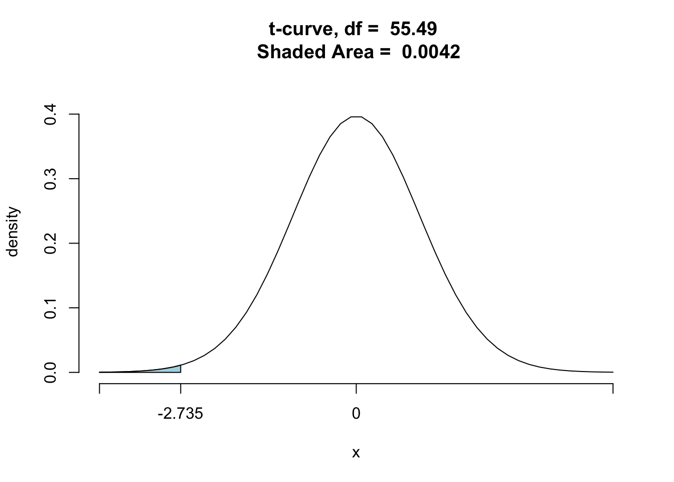
Figure 10.2: P-Value in Two-Sample Test
## [1] 0.00417939710.3.4 Additional Examples
10.3.4.1 A Randomized Experiment
Recall the attitudes experiment. One of the Research Questions we considered back in Chapter Six was the question
Research Question: Does the data provide stronge evidence that the suggested race of the defendant was a factor in the sentence recommended by survey participants?
First, let’s take a look at the data again:
data(attitudes)
View(attitudes)
help(attitudes)
Let’s also remind ourselves of the relationship we found in the data:
favstats(sentence~def.race,data=attitudes)## def.race min Q1 median Q3 max mean sd n missing
## 1 black 3 15 25 40 50 27.77500 14.94891 120 1
## 2 white 4 10 25 40 50 25.84694 15.75602 147 0The defendant whose name suggested he was Black got sentenced to about two years more, on average, than the defendant with the White-sounding name. This goes along with some suspicion we might have that there was some lingering racial prejudice among at least some of the (mostly White) survey participants.
Let us now address our Research Question with a test of significance.
Step One: Define parameters and state hypotheses
As for the parameters, let:
\(\mu_1\) = the mean sentence recommended by all 267 survey participants, if all of the them were to look at a form in which the suggested race of the defendant was Black
\(\mu_2\) = the mean sentence recommended by all 267 survey participants, if all of the them were to look at a form in which the suggested race of the defendant was White
(You may wish to Review Chapter 8 on how to define parameters of interest when an experiment has been conducted).
Now for the hypotheses:
\(H_0\): \(\mu_1-\mu_2 = 0\)
\(H_a\): \(\mu_1-\mu_2 > 0\)
Step Two: Safety Check and Test Statistic
Once again, we begin by running the test code:
ttestGC(sentence~def.race,data=attitudes,
         mu=0,alternative="greater")
Safety Check: It was a matter of chance which participant was assigned which type of survey form, so we conducted a randomized experiment. As for the underlying population being roughly normal, we don’t have to worry about that because the descriptive results in the output shows us that both sample sizes were well above 30:
##  group  mean    sd   n
##  black 27.77 14.95 120
##  white 25.85 15.76 147
As for the test statistic, we see:
## Test Statistic: t = 1.023 The observed difference between the treatment group means is about 1 SD above the value of 0 that the Null expects.
Step Three: P-value
From the output we find that the P-value is 0.1536.
Interpretation of P-Value: If the sentences recommended by the students in the study were, on average, unaffected by the suggested race of the defendant, then there is about a 15.36% chance of getting a test statistic at least a big as the one we got.
Step Four: Decision
Since P > 0.05, we do not reject the Null Hypothesis.
Step Five: Conclusion
This study did not provide strong evidence that the students in the survey were affected by race when they recommended a sentence.
10.3.4.2 A Two-Sided Test
So far all of the tests we have conducted have been one-sided: either the Alternative Hypothesis states that the value of the parameter is GREATER than the Null’s value. or else it says that the parameter is LESS than the Null’s value.
A one sided-test comes along with a one-sided approach to computing a P-value.
For example, when the alternative says GREATER, then the P-value is the chance of the test statistic being equal to or GREATER THAN the value we actually observed for it. On the other hand, when the alternative says LESS, then the P-value is the chance of the test statistic being LESS THAN or equal to the value we actually observed for it.
As a rule, people work with a one-sided Alternative Hypothesis if they have some good reason to suspect—prior to examining the data in the study at hand—that the value of the parameter lies on the side of the Null’s value that is specified by the Alternative. For example, in the “race and recommended sentence” study in the first example of this section, we might have had some prior data or other knowledge that suggests that GC students might be inclined to mete out heavier sentences to a black defendant, and we are using the study to check that view. In that case the one-sided hypothesis would be an appropriate choice.
But suppose that we really don’t have any prior reason to believe that a black defendant would be treated worse, and that we are conducting the study just to see if race makes a difference in sentencing, one way or the other. In that case, a two-sided test of significance might be more appropriate.
Let’s re-do the race and sentencing test, but this time in a two-sided way:
Step One: Define parameters and state hypotheses
This is the same as before. Let
\(\mu_1\) = the mean sentence recommended by all 267 survey participants, if all of the them were to look at a form in which the suggested race of the defendant was Black
\(\mu_2\) = the mean sentence recommended by all 267 survey participants, if all of the them were to look at a form in which the suggested race of the defendant was White
Now for the hypotheses:
\(H_0\): \(\mu_1-\mu_2 = 0\)
\(H_a\): \(\mu_1-\mu_2 \neq 0\)
Step Two: Safety Check and Test Statistic
Safety Check: Same as before. Randomized experiment, large group sizes: we are safe.
For the test statistic, we run the test with the alternative argument set to “two.sided”:
ttestGC(sentence~def.race,data=attitudes,
       mu=0,alternative="two.sided")
##
##
## Inferential Procedures for the Difference of Two Means mu1-mu2:
## (Welch's Approximation Used for Degrees of Freedom)
## sentence grouped by def.race
##
##
## Descriptive Results:
##
## group mean sd n
## black 27.77 14.95 120
## white 25.85 15.76 147
##
##
## Inferential Results:
##
## Estimate of mu1-mu2: 1.928
## SE(x1.bar - x2.bar): 1.884
##
## 95% Confidence Interval for mu1-mu2:
##
## lower.bound upper.bound
## -1.782671 5.638793
##
## Test of Significance:
##
## H_0: mu1-mu2 = 0
## H_a: mu1-mu2 != 0
##
## Test Statistic: t = 1.023
## Degrees of Freedom: 259.1
## P-value: P = 0.3072Again see that t is about 1.02. The observed difference between the treatment group means is about 1 SD above the value of 0 that the Null expects.
Step Three: P-value
This time P-value is 0.3072, as compared to 0.1536 in the one-sided test. What has happened?
In a two-sided test, the P-value is the probability (assuming that the Null is true) of getting a test statistic at least as far from zero (either on the positive or the negative side) as the test statistic that we actually got. Graphically, it looks like Figure [Two-Sided P-Value]:
ptGC(c(-1.02,1.02),region="outside",
     df=259.052,graph=TRUE)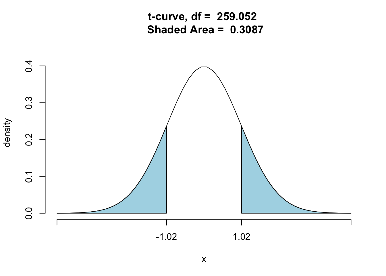
Figure 10.3: Two-Sided P-Value
## [1] 0.3086801Due to the symmetry of the t-curve, a two-sided P-value will generally be twice the corresponding one-sided P-value.
The reason we incorporate both “sides” of the shaded area into the P-value is that at the outset we were indifferent as to whether \(\mu_1=\mu_2\) was positive or negative. The one-sided hypothesis is offered presumably by someone who already has some prior evidence suggesting that the test statistic should turn out a particular way—either positive or negative. Since the P-value measures strength of evidence against the Null, with smaller P-values providing more evidence against the Null, it makes sense that for the same test statistic a one-sided test should return a smaller P-value than a two-sided test. The one sided-test has the evidence from the current data together with some prior evidence, whereas the two-sided test has only the evidence from the current data.
How do we interpret the P-value in a two-sided test? We simply talk about “distance from zero.” So for this study we say:
If the suggested race of defendant has no effect on recommended sentence, then there is about a 30.72% chance of getting a t-statistic at least as far from zero as the one we got in our study.
Step Four: Decision
Since P > 0.05, we do not reject the Null Hypothesis.
Step Five: Conclusion
This study did not provide strong evidence that the students in the survey were affected by race when they recommended a sentence.
10.4 Mean of Differences
In this case we usually have paired data.
10.4.1 Introductory Research Question
Recall the labels data, where participants were asked to rate peanut butter from a jar labeled Jiff, and to rate peanut butter from a jar labeled Great Value, when—unknown to the subjects—both jars contained the same peanut butter.
data(labels)
View(labels)
help(labels)
Recall that subjects tended to rate the Jiff-labeled jar higher:
diff <- labels$jiffrating-labels$greatvaluerating
favstats(diff)
## min Q1 median Q3 max mean sd n missing
## -5 1 2.5 4 8 2.366667 2.809876 30 0But does this data provide strong evidence that the GC population as a whole (not just this sample of 30 students) would rate Jiff higher? In order to address this question, we perform a test of significance:
10.4.2 The Five Steps
Step One: Define parameters and state hypotheses.
The study had a repeated measures design (every participant was measured twice). The parameter of interest is
\(\mu_d\) = mean difference in ratings (Jiff minus Great Value) for ALL Georgetown College students
As for hypotheses:
\(H_0\): \(\mu_d = 0\) (jar makes no difference)
\(H_a\): \(\mu_d > 0\) (Jiff jar rated higher, on average)
We chose the one-sided alternative because Jiff is the more expensive brand, and we have some reasons—based on prior studies about price and perception of quality—to believe that pricier brands are perceived to be of higher quality.
Step Two: Safety Check and Test Statistic.
Hopefully the 30 students in the study were like a random sample from the GC population. The sample size is right at the boundary-value of 30, so let’s go ahead and look at a graph of the sample of differences, checking for strong skewness or big outliers.
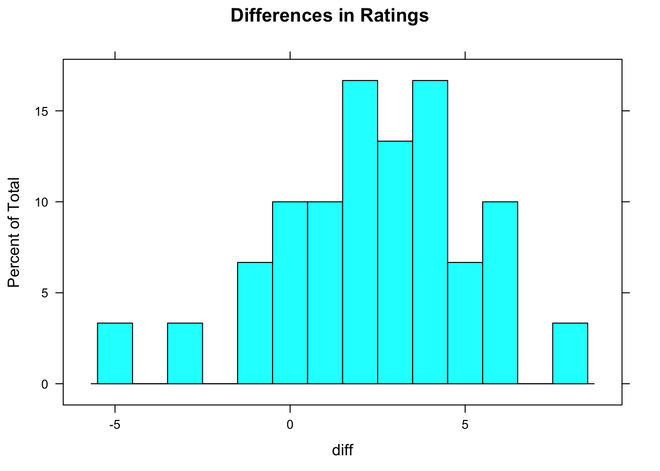
Figure 10.4: Rating Differences
A histogram of the differences is shown in Figure [Rating Differences]. There is a little skewness to the left, perhaps, but not nearly enough to worry about, especially considering our reasonably large sample size. We are safe.
For the test statistic and other information in steps Two through Four, we run ttestGC(), using a special formula-style for matched pairs or repeated-measures data:
ttestGC(~jiffrating-greatvaluerating,
         data=labels,mu=0,alternative="greater")
##
##
## Inferential Procedures for the Difference of Means mu-d:
## jiffrating minus greatvaluerating
##
##
## Descriptive Results:
##
## Difference mean.difference sd.difference n
## jiffrating - greatvaluerating 2.367 2.81 30
##
##
## Inferential Results:
##
## Estimate of mu-d: 2.367
## SE(d.bar): 0.513
##
## 95% Confidence Interval for mu-d:
##
## lower.bound upper.bound
## 1.494996 Inf
##
## Test of Significance:
##
## H_0: mu-d = 0
## H_a: mu-d > 0
##
## Test Statistic: t = 4.613
## Degrees of Freedom: 29
## P-value: P = 3.711e-05The t-statistic is about 4.6133. The mean of the sample differences in ratings is 4.6 SDs above what the Null expects it to be!
Step Three: P-value
Once again, R finds an approximate P-value by using a t-curve (with degrees of freedom one less than the number of pairs in the sample). As we can read from the test output, the P-value is \(3.7 \times 10^{-5}\), or 0.000037 or about 0.00004, which is very small indeed. The interpretation is:
Interpretation of P-Value: If ratings are unaffected by labels, then there is only about 4 in 100,000 chance of getting a t-statistic at least as big as the one we got in our study.
Step Four: Decision
Since P < 0.05, we reject the Null.
Step Five: Conclusion
This data provided very strong evidence that on average people will rate the peanut butter with a more expensive brand-label more highly than the same peanut butter labeled with a less-expensive brand name.
10.4.3 Under the Hood
The formula for the t-statistic is:
\[t = \frac{\hat{d}-\mu_{d,0}}{s_d/\sqrt{n}},\]
where
- \(\hat{d}\) is the mean of the sample differences
- \(\mu_{d,0}\) is what the Null Hypothesis believes \(\mu_d\) is (usually this is 0)
- \(s_d/\sqrt{n}\) is the SE for \(\hat{d}\)
So once again the t-statistic follows the familiar pattern:
\[\text{test statistic} = \frac{\text{observed difference}}{\text{SE for the difference}}.\]
It tells us how many SEs the estimator \(\hat{d}\) is above or below what the Null expects it to be.
This familiar pattern—which applies to each of the three Basic Five parameters involving means—-deserves a name. Let’s call it a z-score-style statistic, since it works like a z-score, measuring the number of SEs the estimator is above or below what the Null expects the parameter to be.
10.4.4 Additional Examples
10.4.4.1 Height and Ideal Height
Recall that in the m111survey participants were asked their height, and the ideal height that they wanted to be. Let’s consider the following
Research Question: Does the study provide strong evidence that, on average, the ideal height of GC students differs from their actual height?
Step One Define Parameter and State Hypotheses
Let
\(\mu_d\) = the mean difference (ideal height minus actual height) for all GC students
Then our hypotheses are:
\(H_0\): \(\mu_d = 0\)
\(H_a\): \(\mu_d \neq 0\)
Note that we have here a two-sided test. Apparently we did not have any prior idea as to whether students want to be taller than they are, on average, or shorter than they are on average.
Step Two Safety Check and Test Statistic
We get the information we need:
ttestGC(~ideal_ht-height,data=m111survey,
         mu=0,alternative="two.sided")
##
##
## Inferential Procedures for the Difference of Means mu-d:
## ideal_ht minus height
##
##
## Descriptive Results:
##
## Difference mean.difference sd.difference n
## ideal_ht - height 1.946 3.206 69
##
##
## Inferential Results:
##
## Estimate of mu-d: 1.946
## SE(d.bar): 0.3859
##
## 95% Confidence Interval for mu-d:
##
## lower.bound upper.bound
## 1.175528 2.715776
##
## Test of Significance:
##
## H_0: mu-d = 0
## H_a: mu-d != 0
##
## Test Statistic: t = 5.041
## Degrees of Freedom: 68
## P-value: P = 3.652e-06There are 69 people who gave usable answers, so the sample is large enough that we don’t have to verify that it looks roughly normal. Also, we are assuming that the sample is like a simple random sample, as far as variables like height are concerned, so we are safe to proceed.
The t-statistic is about 5.04. The sample mean of differences is more than 5 SEs above what the Null expected it to be!
Step Three: P-value
The P-value is \(3.65 \times 10^{-6}\), about 3 in a million.
Interpretation of P-Value: If on average GC students desire to be no taller and no shorter than they actually are, then there is only about a 3 in one million chance of getting a test-statistic at least as far from 0 as the one we got in this study.
Step Four: Decision
P < 0.05, so we reject the Null.
Step Five: Conclusion
This study provided very strong evidence that on average GC students want to be taller than they actually are.
10.4.4.1.1 Tests and Confidence Intervals
In the output from the previous example, look at the confidence interval for \(\mu_d\) that is provided. (Recall that by default it is a 95%-confidence interval.) Notice that it does not contain 0, so according to the way we interpret confidence intervals we are confident that \(\mu_d\) does not equal 0. Of course 0 is what the Null Hypothesis believes \(\mu_d\) is, so we could just as well say that we are confident that the Null is false.
This is an example of a relationship that holds quite generally between two-sided tests and two-sided confidence intervals:
Test-Interval Relationship: When a 95% confidence interval for the population parameter does not contain the Null value \(\mu_0\) for that parameter, then the P-value for a two-sided test
\(H_0\) \(\mu = \mu_0\)
\(H_a\) \(\mu \neq \mu_0\)
will give a P-value less than 0.05, and so the Null will be rejected when the cut-off value \(\alpha\) is 0.05.
Also:
When a 95% confidence interval for the population parameter DOES contain the Null value \(\mu_0\) for that parameter, then the P-value for a two-sided test will give a P-value greater than 0.05, and so the Null will not be rejected when the cut-off value \(\alpha\) is 0.05.
This all makes, sense, because a confidence interval gives the set of values for the population parameter that could be considered reasonable, based on the data at hand. When a particular value is inside the interval, it is reasonable. When outside, it is not reasonable.
The relationship also holds for other confidence levels, provided that you adjust the cut-off value \(\alpha\). In general:
When a \(100 \times(1-\alpha)\)% confidence interval for the population parameter does not contain the Null value \(\mu_0\) for that parameter, then the P-value for a two-sided test will give a P-value less than \(\alpha\).
When a \(100 \times (1-\alpha)\)% confidence interval for the population parameter DOES contain the Null value \(\mu_0\) for that parameter, then the P-value for a two-sided test will give a P-value greater than \(\alpha\).
You may also have noticed that in one sided tests, the ttestGC() function produces one-sided confidence intervals. Recall for example:
t.test(fastest~sex,data=m111survey,mu=0,alternative="less")The one-sided 95% confidence interval extended from negative infinity to -5.17. This interval does not contain zero, which is the Null’s value for \(\mu_1-\mu_2\), and so the Null is rejected with a P-value of less than 0.05.
The relationship between tests and confidence intervals holds not only for two-sided tests and two-sided intervals, but also for one-sided tests and the corresponding one-sided confidence intervals.
10.4.4.2 Repeated Measures, or Two Independent Samples?
Let’s look again at the labels data. By now we are convinced that the data provide strong evidence that GC students (the population from which the data was drawn) are inclined to rate the same product more highly when it is packaged as an “expensive” product that when it as packaged as “cheap”. But notice that in addition to recording the ratings, researchers also recorded the sex of each participant in the study. This raises another interesting research question:
Research Question: Who will be more affected, on average, by the label on a product: a GC female or a GC male?
The original study had a repeated measures design, which resulted in the parameter of interest being a difference of two means. However, when we take sex into consideration things change substantially. Although we still think about the difference between the ratings, we are primarily interested in whether the mean difference for all GC females and the mean differences for all GC guys differ. Thus, the parameter of interest will be a differences of means, where each mean is itself a mean of differences!
Here are the five steps:
Step One: Definition of Parameters and Statement of Hypotheses
Let
\(\mu_d^f\) = the mean difference in rating (Jiff minus Great Value) for all GC females, if all of them could have participated in this study.
\(\mu_d^m\) = the mean difference in rating (Jiff minus Great Value) for all GC males, if all of them could have participated in this study.
The hypotheses are:
\(H_0\): \(\mu_d^f - \mu_d^m = 0\)
\(H_0\): \(\mu_d^f - \mu_d^m \neq 0\)
We chose a two-sided test because we do not have any prior evidence indicating that the difference is positive, or that it is negative.
Step Two Safety Check and Test Statistic
This time we are dealing with two independent (and hopefully random) samples from our two populations. The samples sizes, though, are not so large:
diff <- labels$jiffrating - labels$greatvaluerating[Note that the sample mean difference for the females was a good bit larger than the sample mean difference for the males.]
We have only 15 students in each sample. Since these sample sizes are less than our “safe level” of 30, we really ought to examine them to see if they show signs of strong skewness or outliers.
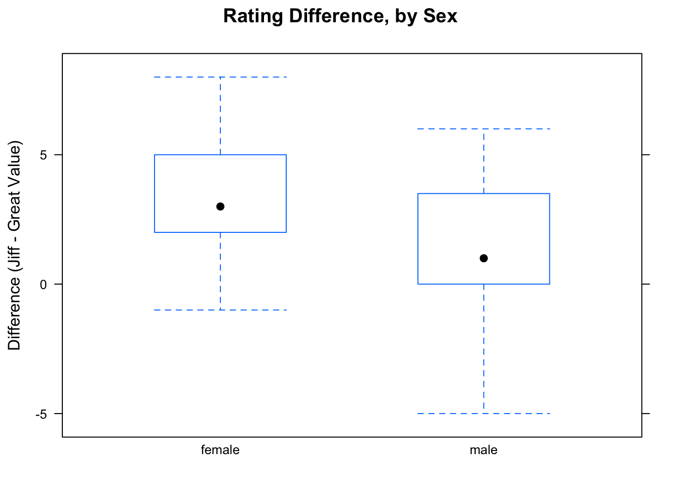
Figure 10.5: Rating Differences for Males and for Females
The results appear in Figure [Rating Differences for Males and Females]. There is some left skewness in the sample of males. We will go ahead and perform the test, but the P-value should be considered a bit dodgy.
For the test, we need to add the differences to our data frame. We accomplish this step as follows:
labels$diff <- diffNow R will recognize diff and process it appropriately, with the usual formula-data input:
ttestGC(diff~sex,data=labels,
         mu=0,alternative="two.sided")
##
##
## Inferential Procedures for the Difference of Two Means mu1-mu2:
## (Welch's Approximation Used for Degrees of Freedom)
## diff grouped by sex
##
##
## Descriptive Results:
##
## group mean sd n
## female 3.533 2.264 15
## male 1.200 2.883 15
##
##
## Inferential Results:
##
## Estimate of mu1-mu2: 2.333
## SE(x1.bar - x2.bar): 0.9465
##
## 95% Confidence Interval for mu1-mu2:
##
## lower.bound upper.bound
## 0.389583 4.277084
##
## Test of Significance:
##
## H_0: mu1-mu2 = 0
## H_a: mu1-mu2 != 0
##
## Test Statistic: t = 2.465
## Degrees of Freedom: 26.51
## P-value: P = 0.02047The value of the t-statistic is 2.47. The observed difference between the sample mean differences for the females and the males is 2.47 SEs above 0 (the value the Null expected it to be).
Step Three: P-value.
The two-sided P-value is 0.02047.
Step Four: Decision
Since P < 0.05, we reject the Null.
Step Five: Conclusion
This data provided strong evidence that GC females are more affected by labels than GC males are.
We might wonder what this all means. Do GC females pay more attention to their surroundings—in particular, to labels on products?? Who knows!
10.5 One Population Proportion
Recall the distribution of the variable sex in the m111survey data:
rowPerc(xtabs(~sex,data=m111survey))##
## sex female male Total
## 56.34 43.66 10056% of the sample—-more than half—were females. This suggests the following:
Research Question: Does this data constitute strong evidence that a majority of the GC student body are female?
10.5.1 The Five Steps
Step One: Definition of Parameter and Statement of Hypotheses
Let
\(p\) = the proportion of females in the GC student population
Then our hypotheses are:
\(H_0\): \(p = 0.50\)
\(H_a\): \(p > 0.50\)
We chose 0.50 as the Null value for \(p\), because we wonder if females are in the majority (proportion bigger than 0.5) at GC. Choosing the Null in this way allows the Alternative to express the idea that females are in the majority. If we had let the Null say something else (\(p= 0.48\) for example) then the Alternative (\(p > 0.48\)) would leave a bit of room for females NOT be in the majority.
Step Two: Safety Check and Test Statistic
As with confidence intervals for one population proportion, the safety check for significance tests includes thinking about whether our sample is like a simple random sample—at least with respect to the variables we are measuring. In this study, our sample consists of all the students taking MAT 111 in a given semester. Now people often take MAT 111 for reasons connected to the requirements of their prospective major. If the two sexes differ with regard to what majors they prefer, then this sample could be a biased one. On these grounds, our test is going to be a bit untrustworthy.
Let’s go ahead and run the test. As with confidence intervals, when we are interested in a single proportion we can use binomtestGC().
binomtestGC(~sex,data=m111survey,p=0.5,
            alternative="greater",success="female")
## Exact Binomial Procedures for a Single Proportion p:
## Variable under study is sex
##
## Descriptive Results: 40 successes in 71 trials
##
## Inferential Results:
##
## Estimate of p: 0.5634
## SE(p.hat): 0.0589
##
## 95% Confidence Interval for p:
##
## lower.bound upper.bound
## 0.458929 1.000000
##
## Test of Significance:
##
## H_0: p = 0.5
## H_a: p > 0.5
##
## P-value: P = 0.1712Notice what we had to do in order to get all that we needed for the test:
- we had to specify the Null value for \(p\) by using the
pargument; - we had to set
alternativeto “greater” in order to accommodate our one-sided Alternative Hypothesis; - we had to say what the proportion is a proportion of: is it a proportion of females or a proportion of males? We accomplished this by specifying what we considered to be a success when the sample was tallied. Since we are interested in the proportion of females, we counted the females as a success, so we set the
successargument to “female”.
Looking at the output, you might wonder what the test statistic is. In binomtestGC(), it’s pretty simple: it’s just the number of females: 40 out of the 71 people sampled.
Step Three The P-value
This is 0.1712. It is the probability of getting at least 40 females in a sample of size 71, if the population consists of 50% females. So we might interpret the P-value as follows:
Interpretation of P-Value: If only half of the GC population is female, then there is about a 17% chance of getting at least as many females (40) as we actually got in our sample.
Step Four Decision
We do not reject the Null, since the P-value is above our standard cut-off of 5%.
Step Five: Conclusion
This survey data did not provide strong evidence that females are in the majority at Georgetown College.
10.5.2 Under the Hood
Note that the test statistic did not follow the “z-score” pattern of the three previous tests involving means. The test statistic is simply the observed number of successes.
binomtestGC() gets its P-value straight from the binomial distribution. If we wanted, we could get the same P-value using the familiar pbinomGC function:
pbinomGC(39,region="above",size=71,prob=0.5)It may be worth recalling that, as with any test function in the tigerstats package, you can get a graph of the P-value simply by setting the argument graph to TRUE:
binomtestGC(~sex,data=m111survey,p=0.5,
            alternative="greater",success="female",
            graph=TRUE)
Now we know from Chapter 7 that when the number of trials \(n\) is large enough, then the distribution of a binomial random variable looks very much like a normal curve. In fact, when this is so, binomtestGC() will actually use a normal curve to approximate the P-value!
There is another test that makes use of the normal approximation in order to get the P-value, and it is encapsulated in the proptestGC() function:
proptestGC(~sex,data=m111survey,p=0.50,
        alternative="greater",success="female")
##
##
## Inferential Procedures for a Single Proportion p:
## Variable under study is sex
## Continuity Correction Applied to Test Statistic
##
##
## Descriptive Results:
##
## female n estimated.prop
## 40 71 0.5634
##
##
## Inferential Results:
##
## Estimate of p: 0.5634
## SE(p.hat): 0.05886
##
## 95% Confidence Interval for p:
##
## lower.bound upper.bound
## 0.466564 1.000000
##
## Test of Significance:
##
## H_0: p = 0.5
## H_a: p > 0.5
##
## Test Statistic: z = 0.9571
## P-value: P = 0.1692Here the test statistic is
\[z=\frac{\hat{p}-p_0}{\sqrt{\frac{\hat{p}(1-\hat{p})}{n}}},\]
where
- \(\hat{p}\) is the sample proportion,
- \(p_0\) is the Null value of \(p\),
- the denominator is the standard error of \(\hat{p}\).
Like the test statistics for means, it is “z-score style”: it measures how many standard errors the sample proportion is above or below what the Null Hypothesis expects it to be.
When the sample size is large enough and the Null is true, the distribution of this test statistic is approximately normal with mean 0 and standard deviation 1. in other words, it has the standard normal distribution. Therefore the P-value comes from looking at the area under the standard normal curve past the value of the test statistic. (We also apply a small continuity correction in order to improve the approximation; consult GeekNotes for details.)
Many people will say that the sample should contain at least 10 successes and 10 failures in order to qualify as “big enough.” (The binomtestGC() gives an “exact” P-value and is not subject to this restriction.)
For tests involving a single proportion, you may use either proptestGC() or bimom.testGC(). The choice is up to you, but we have a slight preference for binom.testgC(), since it delivers “exact”" P-values regardless of the samples size.
10.5.3 Additional Examples
10.5.3.1 An ESP Experiment: Summary Data, and Care in Drawing Conclusions
The following example deals with a study that was actually conducted at the University of California at Davis around the year 1970.
The researcher, a para-psychologist named Charles Tart, was looking for evidence of extrasensory perception (ESP) in human beings. Tart designed a machine that he called the “Aquarius”, which could generate numbers. He set the machine to generate either 1, 2, 3, or 4. For each subject in the study, the Aquarius machine generated 500 numbers, and after each number was generated the subject was asked to guess the number. After each guess was submitted, the machine would show the subject the “correct” number by flashing one of four numbered lights, and then would generate the next number.
One study involved fifteen subjects, who made a total of
\[15 \times 500 = 7500\]
guesses. Out of this total, 2006 of the guesses were correct.
Let’s think about these results. If the subjects have no ESP at all, then it would seem that they would be reduced to guessing randomly, in which case the chance of a correct guess should be 1 in 4, or 0.25. Then the number \(X\) of correct guesses in these 7500 tries would be a binomial random variable, with \(n=7500\) trials and chance of success \(p=0.25\). The expected number of correct guesses would then be:
\[np = 0.25 \times 7500 = 1875.\]
The observed number of correct guesses was 2006, which is 131 more than expected. We wonder if this observation constitutes strong evidence that at least some of the subjects had at least some ESP powers.
Let’s try a test of significance to find out:
Step One: Define Parameter and State Hypotheses.
Let
\(p\) = probability that a subject will guess correctly.
Then our hypotheses are:
\(H_0\): \(p = 0.25\)
The Null expresses the view that the subjects have no ESP; they are just randomly guessing.
\(H_a\): \(p > 0.25\)
The Alternative expresses the view that the subjects can do something better than guess randomly.
Step Two: Safety Check and Test Statistic.
The test statistic is easy: it’s the 2006 correct guesses. As for the safety check: we are not picking from a population so we don’t have to check whether we have taken a simple random sample from a population. If the Null is right, the subjects are just guessing randomly, so the number of correct guesses would be binom(7500,0.25), as explained above.
Step Three: P-value
Let’s run the test. we have summary data, so we don’t have to specify what counts as a success; we only need to enter the number of successes and the number of trials:
binomtestGC(2006,n=7500,p=0.25,alternative="greater")## Exact Binomial Procedures for a Single Proportion p:
## Results based on Summary Data
##
## Descriptive Results: 2006 successes in 7500 trials
##
## Inferential Results:
##
## Estimate of p: 0.2675
## SE(p.hat): 0.0051
##
## 95% Confidence Interval for p:
##
## lower.bound upper.bound
## 0.259061 1.000000
##
## Test of Significance:
##
## H_0: p = 0.25
## H_a: p > 0.25
##
## P-value: P = 3e-04Hmm, the P-value is very small: about 0.0003.
Interpretation of P-Value: If all of the subjects had only a 25% chance of guessing correctly, then there is only about a 3 in 10,000 chance that they would get a total of at least 2006 correct guesses, as they did in this study.
Step Four: Decision
We reject the Null, since the P-value was so very small.
Step Five: This study provided very strong evidence that at least some of the subjects in the study had more than a 1-in-4 chance of guessing correctly.
Notice how carefully the conclusion was framed, in terms of the probability of a correct guess rather than whether or not anyone has ESP. The reason for this caution is that the test of significance only addresses the mathematical end of things: in particular, it does not address whether the study was designed well enough so that a \(p\) being larger than 0.25 would be the very same thing as some subjects possessing ESP powers.
It turned out, in fact, that there was a problem with the design of the study: the machine’s random-number generation program was defective, in such a way that it rarely generated the same number twice in a row. Some of the subjects probably recognized this pattern and adopted the strategy of guessing randomly one of the three numbers that had not been generated in the previous round. These subjects would then improve their chance to 1-in-3 for the rest of their trials.
There is an important moral to this story:
A significance test only tells you whether or not it is reasonable to believe that the results could be obtained by chance if the Null is true. It does NOT tell you how the Alternative Hypothesis should be interpreted. When the study has a flawed design, the results of the test will not mean what you expect them to mean!
10.6 Difference of Two Proportions
Recall that in the mat111survey, participants were asked their sex, and were also asked whether they believed in love at first sight. The results were as follows:
SexLove <- xtabs(~sex+love_first,data=m111survey)
rowPerc(SexLove)
## love_first
## sex no yes Total
## female 55.00 45.00 100.00
## male 74.19 25.81 100.00In the sample, the females were much more likely than the males to believe in love at first sight (45% vs. 25.81%), but these figures are based on fairly small samples. We wonder whether they provide strong evidence that in the GC population at large females are more likely than males to believe in love at first sight.
Now this is a question about the relationship between two categorical variables, so we could address it with the chi-square test from Chapter 3:
chisqtestGC(SexLove)However, when the explanatory and reponse variables both have only two values, then it is possible to construe the question as a question about the difference between two proportions. A two-proportions test confers some advantages in terms of how much information we extract from the data.
10.6.1 The Five Steps
Step One: Definition of Parameters and Statement of Hypotheses
Let
\(p_1\) = the proportion of all GC females who believe in love at first sight
\(p_2\) = the proportion of all GC males who believe in love at first sight
The our hypotheses are:
\(H_0\): \(p_1 - p_2 = 0\)
\(H_a\): \(p_1 - p_2 > 0\)
Step Two: Safety Check and Test Statistic
The Safety Check is the same as for confidence intervals:
- We should have taken two independent simple random samples from two populations, OR we should have done a completely randomized experiment with two treatment groups;
- the sample size should be “large enough” (see below).
In this current case, we have two samples from two populations (the GC gals and the GC guys). There is some concern as to whether the samples are really “like” simple random samples, but since one’s decision to take MAT111 (and hence get into the survey) is probably unrelated to whether one believes in love at first sight, maybe we can count ourselves as “safe” on this point.
As for a “large enough” sample size, we plan to use proptestGC(), just as we used it to make confidence intervals for \(p_1-p_2\). Hence the safety criteria are the same: if the number of yesses and nos in both samples exceeds 10, then we can trust the approximation to the P-value that the test provides. If in one of the samples there are not at least ten yesses, and not at lest ten nos, then the computer will issue a warning.
proptestGC(~sex+love_first,data=m111survey,
        success="yes",p=0,alternative="greater")
The descriptive results are given first:
##        yes  n estimated.prop
## female  18 40         0.4500
## male     8 31         0.2581
From these results we can see that there are fewer than ten males who answered “yes”, and sure enough the routine delivers its warning:
## WARNING:  In at least one of the two groups,
## number of successes or number of failures is below 10.
## The normal approximation for confidence intervals
## and P-value may be unreliable.
For the sake of seeing the entire example, we will proceed anyway.
When we come to the inferential results, we see the estimator \(\hat{p}_1-\hat{p}_2\), and the standard error of this estimate:
## Estimate of p1-p2:   0.1919
## SE(p1.hat - p2.hat):  0.1112
Note that the estimate is not even two standard errors above the value of 0 that the Null expects it to be. The results of this study are not very surprising, if the Null is in fact correct.
The formula for the test statistic is:
\[z=\frac{\hat{p}_1-\hat{p}_2}{\sqrt{\frac{\hat{p}_1(1-\hat{p}_1)}{n_1}+\frac{\hat{p}_2(1-\hat{p}_2)}{n_2}}},\]
so once again it has “z-score style”, telling us how many SEs the estimator is above or below the 0 that the Null expects. In this case its numerical value, according to the output, is:
## Test Statistic: z = 1.726 Step Three: P-Value
The output says that the P-value for the one-sided test is:
## P-value: P = 0.04216According to this test, if in the GC population females are equally likely to believe in love at first sight, then there is about a 4.2% chance for the differences between the sample proportions (45%-25.8%) to be at least a big as it was observed to be.
Step Four: Decision
Since \(P = 0.042 < 0.05\), we reject the Null.
Step Five: Conclusion
This data provided strong evidence that GC females are more likely than GC males to believe in love at first sight.
We stress, though, that we completed the test in the presence of a warning from R. There do exist other routines that attempt to provide better approximations to the P-value when samples are small, and they result in somewhat different conclusions. (One such test is prop.test(); see the GeekNotes.)
10.6.2 Working With Summary Data
Imagine an experiment in which there are 2000 subjects who are randomly divided into two groups of size 1000 each. All subjects get a shot in mid-October. Member of Group A (control) gets a shot that feels just like getting a flu vaccine but which actually delivers an inert substance, whereas every member of group B gets a shot containing the current flu vaccine. (Note the blinding.) Doctors monitor the subjects until Spring, and record whether or not each subject caught the flu. Of the 1000 members of Group A, 80 got the flu, whereas of the 1000 members of Group B, 40 got the flu. We are interested in the following:
Research Question: Do the results provide strong evidence that the flu vaccine was effective in reducing the risk of flu that year?
We have summary data, so we use proptestGC() for summary data just as we did for confidence intervals.
Step One: Define parameters and state hypotheses.
Let:
\(p_1\) = the proportion of all 2000 subjects who would have caught the flu, if all of them had been given the inert substance
\(p_2\) = the proportion of all 2000 subjects who would have caught the flu, if all of them had been given the real flu vaccine
Then the hypotheses are:
\(H_0\): \(p_1-p_2 = 0\)
\(H_a\): \(p_1-p_2 > 0\)
Step Two: Safety Check and Test Statistic
Let’s run the test:
- We need to tell R the number of successes in the two samples, and we do this by putting
c(80,40)into an argument calledx. - We also need to tell R the sample sizes, so we put
c(1000,1000)into an argument calledn. - We tell R that the Null thinks \(p_1-p_2\) is 0, by setting an argument
pto 0. - Finally, we tell R what the alternative hypothesis looks like, by setting
alternativetotwo.sided:
proptestGC(x=c(80,40),n=c(1000,1000),
          p=0,alternative="two.sided")
##
##
## Inferential Procedures for the Difference of Two Proportions p1-p2:
## Results taken from summary data.
##
##
## Descriptive Results:
##
## successes n estimated.prop
## Group 1 80 1000 0.08
## Group 2 40 1000 0.04
##
##
## Inferential Results:
##
## Estimate of p1-p2: 0.04
## SE(p1.hat - p2.hat): 0.01058
##
## 95% Confidence Interval for p1-p2:
##
## lower.bound upper.bound
## 0.019258 0.060742
##
## Test of Significance:
##
## H_0: p1-p2 = 0
## H_a: p1-p2 != 0
##
## Test Statistic: z = 3.78
## P-value: P = 0.0001571There was no warning, so the sample sizes were big enough. Also, we did a randomized experiment, so we are safe to proceed.
The test statistic is \(z=3.78\), indicating that the difference in sample proportions (8% in the control group vs. 4% in the vaccine group) was about 3.78 standard errors bigger than the Null expected it to be.
Step Three: P-value
The P-value was quite small, about 0.00016.
Interpretation of P-Value: If the vaccine is doing no good, then there is only about a 16 in 100,000 chance of getting a test statistic at least as far from 0 as the one we got in our study.
Step Four: Decision
Since \(P=0.00016 < 0.05\), we reject the Null.
Step Five: Conclusion
This experiment provided strong evidence that the vaccine helps to prevent flu.
By the way: if the vaccine was effective, why was it not perfect? 40 out of 1000 people using the vaccine got the flu anyway! There are two reasons why flu vaccines are not completely effective:
- The flu vaccine is based on a “dead virus”, so it takes a while—usually about two weeks—for the body to recognize its existence and to develop the appropriate antibodies. During that period a person who is exposed to the flu could easily “catch” it.
- The flu vaccine is designed each year by scientists at the Center for Disease Control, who make the best prediction they can as to which strains of flu are most likely to be prevalent in the coming winter. The vaccine is based on these strains, and is not guaranteed to work against all possible strains to which a person might be exposed.
10.7 Further Considerations About Significance Tests
As we have covered each of the Basic Five in this Chapter and in Chapter Three, we have run across ideas that apply to all significance tests. Here is a quick rundown of what we have learned so far:
- The Five-Step logic applies to all significance tests.
- If your test concerns one or more parameters, then you need to define your parameters and then use the symbols for those parameters to state your hypotheses.
- The hypotheses always talk about what’s going on in the population(s), not the samples. (If we did an experiment, then the hypotheses talk about what would happen if all the subjects were given each of the treatments.)
- The Null is the hypothesis that says that there is no pattern in the population.
- The Alternative always involves an inequality.
- Tests involving one of the Basic Five can be either one-side or two-sided. This affects the computation of P-values.
- It’s always useful to stop and think about the test statistic. With the exception of
binomtestGC()the test statistic is “z-score style”, and it tells you how many SEs the estimator is above or below what the Null expects. When it is far from 0, that’s bad for the Null! - P-values can always be interpreted according to following format: If [the Null is True], then there is about a [P-value] chance of getting a test statistic at least as extreme as the one we actually got in this study.
- We can run tests straight from a data frame using formula-data input, or we can enter summary data.
- Tests only check the Null Hypothesis in mathematical form. They don’t check whether the study was well-designed (see the ESP example).
- There is a correspondence between tests and confidence intervals that basically says: when the interval does not contain the Null’s belief about the parameter, then the test will reject the Null, and when the interval contains the Null’s belief the test will not reject the Null.
There are some additional concepts that apply to all significance tests, and in this section we will consider some of them.
10.7.1 Types of Error
There is no guarantee that Step Four (the Decision) in a test of significance will be correct. That’s because the sample is based on chance. No matter how much the sample estimator for the population parameters differs from what the Null expects it to be, the difference COULD POSSIBLY be due to our having drawn a really rare, unlikely sort of sample. So even when we reject the Null based on a low P-value, the Null could be correct anyway. The error that we make in such a situation is called a Type-I Error.
It goes the other way around, too: we might fail to reject the Null when it is in fact false. Such an error is called a Type-II Error.
The fact that a test can deliver an error is not a sign that the testing procedure is bad. On the contrary, just as a well-designed formula for a 95%-confidence interval SHOULD fail to contain the population parameter 5% of the time in repeated sampling, so a well-designed test of significance with a 5% cut-off standard SHOULD commit a Type-I error 5% of the time in repeated sampling, if the Null is in fact correct.
The only way never to commit a Type-I error is to NEVER reject the Null. But if that’s your plan, then you might as well not collect any data at all: it won’t affect your decision about the Null Hypothesis!
When the Null is false, you are correct when you reject the Null. The probability of rejecting the Null when it is, in fact, false is called the power of the test. The power depends on “how false”" the Null actually is. The more the Null’s belief about the parameter differs from what the parameter actually is, the higher the power should be.
Sample size makes a difference, too. If the Null is, in fact, false then you are more likely to be able to detect that fact using a large sample than you are using a small one. Tests that are based on large samples are therefore more powerful than tests based on small samples.
The app below illustrates the idea we have broached concerning Type-I and Type-II errors. The app draws random samples from a population that is normally distributed, computes a confidence interval based on the sample, and performs a two-sided test for the mean of the population, too.
In all scenarios, the true mean of the population is \(\mu = 170\).
When you choose to draw one sample per mouse click, you will see a histogram of of the sample in blue. You will also see a confidence interval in yellow, with the sample mean as a blue dot in the middle of that interval. In the console, you will get the results of a two-sided test for where the null says that \(\mu\) is 170 (that is, \(\mu_0=170\)). You can vary the true population mean \(\mu\) with a slider.
require(manipulate)
Type12Errors()
To start out, keep the true population mean \(\mu\) set at 170, so that the null is actually true. This means that whenever the tests rejects the Null, a Type-I error has been made. Click through a number of samples one at a time. Then try many samples (a hundred, or a thousand). What proportion of the time do you get a Type-I error?
Next, move the \(\mu\) slider a bit away from 170. Now the Null is false, so whenever you reject it you have not made an error. Try lots of samples: what happens to the proportion of rejections, in the long run, after many samples?
Next. keeping \(\mu\) where it is, move up the sample size \(n\), and run one sample at a time. What happens to the confidence intervals: are they wider than before, or narrower? What proportion of the time do you correctly reject the Null? Is it higher or lower than it was when the sample size was smaller?
Some Basic Ideas Learned From the the App:
- The test is designed so that if the Null is true and your cut-off value (aka level of significance) is \(\alpha\), then the test will incorrectly reject the Null (i.e. commit a Type-I Error) \(100\alpha\) percent of the time.
- The further the Null’s belief is from the actual value of the population parameter, the more likely it is that the test will reject the Null (i.e., the more powerful the test is).
- The bigger the sample size, the more powerful the test will be when the Null is false. When the sample size is very large, even a Null that is only a “little bit” false is quite likely to be rejected.
The last point is especially important. When the sample size is very large, the test is very likely to detect the difference between a false Null belief and the true parameter value, even when the two are very close together. A large-sample test can thus provide strong evidence for what amounts to a very weak pattern in the population. Hence you should always keep in mind:
Strong evidence for a relationship is not the same thing as evidence for a strong relationship.
10.7.2 The Dangers of Limited Reporting
Suppose that you have twenty friends, and you are interested in knowing whether any of them possess powers of telekinesis (TK for short). Telekinesis (if such a thing exists at all) is the ability to move objects by mental intention alone, without touching them.
You perform the following test with each of your friends: you flip a fair coin 100 times, after instructing your friend to attempt to make the coin land Heads simply by concentrating on it.
You get the following results:
CoinData## heads
## 1 57
## 2 54
## 3 57
## 4 61
## 5 45
## 6 52
## 7 60
## 8 52
## 9 48
## 10 57
## 11 58
## 12 58
## 13 51
## 14 46
## 15 49
## 16 53
## 17 51
## 18 51
## 19 48
## 20 46Hmm, one of your friends (Friend Number Four) got 61 Heads in 100 flips. That seems like a lot. If your friend has no TK—so that the coin has the usual 50% chance of landings heads—then the chance of 61 or more heads is pretty small:
pbinomGC(60,region="above",size=100,prob=0.5)## [1] 0.0176001If you run a binomtestGC() on your friend’s results, you get the same information:
Step One: Define Parameter and State the Hypotheses
Let
\(p\) = chance that coin lands Heads when Friend Number Four concentrates on it.
The hypotheses are:
\(H_0\): \(p = 0.50\) (Friend #4 has no TK powers)
\(H_a\): \(p > 0.50\) (Friend #4 has some TK powers)
Step Two: Safety Check and Test Statistic
We flipped the coin randomly so we are safe. The test statistic is 61, the number of Heads our friend got.
Step Three: P-value
binomtestGC(61,n=100,p=0.5,alternative="greater")## Exact Binomial Procedures for a Single Proportion p:
## Results based on Summary Data
##
## Descriptive Results: 61 successes in 100 trials
##
## Inferential Results:
##
## Estimate of p: 0.61
## SE(p.hat): 0.0488
##
## 95% Confidence Interval for p:
##
## lower.bound upper.bound
## 0.523094 1.000000
##
## Test of Significance:
##
## H_0: p = 0.5
## H_a: p > 0.5
##
## P-value: P = 0.0176Sure enough, the P-value is 0.0176.
Step Four: Decision
Since P < 0.05, we reject the Null.
Step Five: Conclusion
Our data (the 100 coin flips in the presence of Friend Number Four) provide strong evidence that when Friend Four concentrates on this coin he/she has more than a 50% chance of making it land Heads.
There is nothing wrong with any step in this test, and yet it seems quite wrong to conclude that Friend Number Four actually has some TK powers.
Why? Because your friend was only one of twenty people tested. When you test a lot of people, then even if none of them have TK you would expect a few of them to get an unusually large number of heads, just by chance, right?
Just as with any test of significance, binomtestGC() considers ONLY the data that you present to it. When it is allowed to consider ONLY the results from Friend Number Four, R leads you to a perfectly reasonable conclusion: those 100 flips, when considered in isolation from other data, provide strong evidence for some TK powers in Friend Four.
But it’s not right to consider the 100 flips in isolation. Instead, should we not at least take into account that our friend’s results were the maximum out of a study involving twenty friends?
Perhaps a more relevant P-value for this situation—one that takes more of the data into account—is the probability of at least one person getting 61 or more heads when 20 people, none of whom have TK, participate in a study like this.
If you run the following R code, you will teach R a function that conducts the entire study and returns the maximum number of heads achieved by any friend
HeadMax <- function(friends=20,flips=100,coin=0.5) {
  return(max(rbinom(friends,size=flips,prob=coin)))}
Now run the function:
HeadMax(friends=20,flips=100)Re-run the function a number of times. Do you notice that it is not such a rare thing at all for at least one person to get at least 61 heads?
In fact, if you were to run the function many times and keep track of the results, you would find that—even if there is no such thing as TK—there is about a 30% chance that at least one friend will get 61 or more heads. When you think of it this way, you see that 61 heads is not strong evidence for TK!
The moral of the story is this:
Tests of significance consider only the data presented to them.
If you use a test that is based on only a limited portion of the data, the test does not deliver meaningful results. Instead:
- Report all relevant data you have collected.
- Look for ways to incorporate all of the relevant data when you are testing for statistical significance.
10.7.3 The Dangers of Data-Snooping
The example in the previous section may seem somewhat artificial. After all, you are an honest-to-good scientist—or at least you are planning to take some honest-to-good science classes—and you know that real, honest scientists do not knowingly limit their reporting to just those portions of the data that point in an interesting direction.
But it’s amazing how much we can limit our reporting without even knowing it.
For example, consider the attitudes data. If you need a reminder, run:
data(attitudes)
View(attitudes)
help(attitudes)
As you will recall, there was a limited number of primary research questions that guided the design of the attitudes study:
- Does suggested race of defendant affect the sentence recommended?
- Does suggested race of victim affect the sentence recommended?
- Does the way one lost one’s money affect the decision about whether to attend the concert anyway?
But the researchers could not resist the urge to collect some other information beyond what was needed to narrowly address the primary research questions. For example, the researcher got information on the sex, class rank and intended major of each participant.
There is nothing wrong at all with the urge to collect extra data. In fact it’s a wonderful human trait, is it not?
And of course there is nothing at all wrong with the urge to explore the data thus collected. It’s a rich data set (there are a lot of variables), so there are many research questions one could raise.
For example, we might explore the
Research Question: Who is harder on crime: a GC female or a GC male?
When you think about the kinds of variables involved in this question (explanatory = sex is a factor, response = sentence is numerical) you see that favstats() will provide useful descriptive statistics:
favstats(sentence~sex,data=attitudes)## sex min Q1 median Q3 max mean sd n missing
## 1 female 3 15.0 25 40 50 27.30793 15.46790 164 1
## 2 male 3 12.5 25 40 50 25.76699 15.31832 103 0Hmm, nothing much seems to be going on here.
Let’s try another
Research Question: Who is more likely to decide to attend the rock concert anyway: a GC female or a GC male
Again, we work our way from research question to variable to type of each variable to exploration technique and we hit upon the following R code:
SexRock <- xtabs(~sex+conc.decision,data=attitudes)
SexRock
## conc.decision
## sex buy not.buy
## female 112 53
## male 64 39rowPerc(SexRock)## conc.decision
## sex buy not.buy Total
## female 67.88 32.12 100.00
## male 62.14 37.86 100.00Hmm, apparently there not much going on in the way of a relationship between sex and decision to attend a rock concert.
Still another
Research Question: Who is harder on crime: A GC student who would decide to atttend the rock concert or a GC student who decide not to attend?
Again we check:
favstats(sentence~conc.decision,data=attitudes)## conc.decision min Q1 median Q3 max mean sd n missing
## 1 buy 3 15 25 45 50 28.15143 15.70951 175 1
## 2 not.buy 3 10 20 30 50 23.97826 14.48453 92 0Interesting: in the survey those who chose to attend (let’s call them “Big Spenders”) recommended sentences for the defendant that were, on average, five years longer than the sentences recommended by the Thrifty types—the ones who chose not to attend.
Let’s check it out graphically: Figure [Sentences and Ticket Decision] shows the results. The plot thickens! The distributions are fairly similar in shape, but it appears that the Big Spender group had a substantially higher proportion of people who recommended the maximum sentence of 50 years: that pulled up their mean sentence.
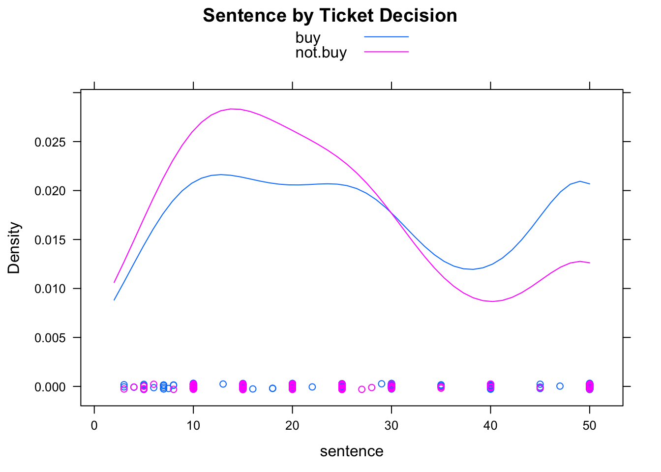
Figure 10.6: Sentence and Ticket Decision
Let’s test to see if these results are statistically significant. We won’t write out all five steps, but instead let’s just peek at the test output. (We’ll choose a two-sided test, because we had no advance evidence that Big Spenders should be harder on crime that Thrifty people.)
ttestGC(sentence~conc.decision,data=attitudes,
         mu=0,alternative="two.sided")
##
##
## Inferential Procedures for the Difference of Two Means mu1-mu2:
## (Welch's Approximation Used for Degrees of Freedom)
## sentence grouped by conc.decision
##
##
## Descriptive Results:
##
## group mean sd n
## buy 28.15 15.71 175
## not.buy 23.98 14.48 92
##
##
## Inferential Results:
##
## Estimate of mu1-mu2: 4.173
## SE(x1.bar - x2.bar): 1.921
##
## 95% Confidence Interval for mu1-mu2:
##
## lower.bound upper.bound
## 0.384772 7.961563
##
## Test of Significance:
##
## H_0: mu1-mu2 = 0
## H_a: mu1-mu2 != 0
##
## Test Statistic: t = 2.172
## Degrees of Freedom: 198.6
## P-value: P = 0.03102Hmm, the P-value is about 0.03. It appears that we have some strong evidence here that GC Big Spenders are harder on crime than GC Thrifties are.
Do you see what’s going on here? We have followed a natural and perfectly commendable human urge to paw through the available data, formulating research questions as we go and investigating them with appropriate descriptive techniques, deciding to run an inferential test only when descriptive techniques turned up an interesting pattern in the data. Although our intentions were quite honest, we are acting very much like the person in the previous section who decided to run binomtestGC() on the one friend who “produced” an intriguingly-large number of heads! This time, though, instead of testing on a limited amount of relevant data, we are testing on a limited number of aspects of the data. We are looking at the data from many different angles, as it were, and choosing to test on the angles that look “pretty”.
Even a totally ordinary piece of furniture (for example) can look “pretty” from a particular point of view, in a particular light, etc.
This practice—pawing through a rich data set, examining it from different points of view and performing tests on the basis of interesting patterns that we happen to notice when looking at the data from some of those vantage points—is called data-snooping.
- Data Snooping
Data Snooping is the practice of looking through a data set for patterns that interest us and performing inferential procedures on patterns that we notice, rather than limiting our tests to specific Research Questions that we had in mind prior to collecting the data.
Data snooping is not an inherently evil practice: on the contrary, it is an expression of two excellent human traits: curiosity, and the ability to detect many types of patterns. The problem is that the more curious we are, and the better we are at noticing patterns, the more likely it is that our data-snooping will lead us to report results as statistically significant when in fact they are only due to random quirks in the data.
The problem is especially acute because—unlike the “limited reporting” example of the previous section, where we can correct ourselves by taking all of the data into account—we don’t really know what kinds of patterns we as humans are disposed to find intriguing: we don’t know what constitutes the “set of all aspects” that have to be taken into account when one attempts to adjust the P-values for the tests on those particular aspects that, for one reason or another, got us excited.
This is really interesting: we have identified a problem in how to assess rationally what our observations entail, but this problem does not arise from our not knowing something about how the data was collected, nor does it arise from our not knowing something about the population. It arises from our not knowing something about ourselves.
There is no fool-proof solution to the problem of data-snooping. As a general rule of thumb, though, we should keep clearly in mind the distinction between:
- those research questions that we had in mind prior to collecting the data (Primary Questions) versus
- those research questions that occur to us as we examine the collected data in all of its richness (Secondary Questions).
Results of tests on Primary Questions should be taken more seriously than results of tests on Secondary Questions. The Results for Secondary Questions may be worth reporting to others (especially if they provide exceedingly strong evidence for a pattern), but we should be clear when we report them that the results were based on patterns that we noticed AFTER having examined the data. Perhaps in the future other researchers could treat them as Primary Questions, should they conduct a study similar to ours. If the same pattern persists in study after study, then we can be more and more certain that it is not due to chance variation in the data collection process, but reflects instead a pattern in the population itself.
10.8 Thoughts About R
10.8.1 New Code to Learn?
Functions for tests are the same as for confidence intervals! However, you have to consider some additional arguments. You need to pay attention to:
- the argument that sets the Null value for the parameter:
muin tests involving meanspin tests involving proportionsprobinbinomtestGC()
- the
alternativeargument that specifies the “side” of the test- “greater”
- “less”
- “two.sided”
The default value of alternative is “two.sided”, so if you want a two-sided test you need not mention alternative in your call to the function. For example, the following two functions calls will deliver exactly the same results:
ttestGC(~fastest,data=m111survey,
       mu=100)
ttestGC(~fastest,data=m111survey,
       mu=100,alternative="two.sided")
10.8.2 Old Descriptive Friends
When you perform safety checks in the tests involving means and you have access to the original data rather than just a summary of it, then you may have to make graphs of your samples in order to check for skewness and outliers. For this you will revisit some old friends from Chapter Two. You should be fine with:
histogram()bwplot()
10.8.3 Adding a Variable to a Data Frame
On rare occasions you may need to add a variable to a data frame prior to running a test involving that variable. This occurred to us once, in the Research Question about whether women or men are more affected by the label on a jar of peanut butter. In order to add a variable Var to a data frame MyData, simply write:
MyData$Var <- VarThe length of Var must be the same as the number of rows in the data frame.