Chapter 11 Goodness of Fit
At the beginning of Chapter Two our very first foray into Descriptive Statistics concerned exploring the distribution of a single factor variable. In this Chapter we will introduce a way to address inferential aspects of Research Questions about one factor variable.
11.1 The Gambler’s Die
Imagine that you are the Sheriff of a small town in the Wild, Wild West. A professional gambler comes to town, and sets up shop in the local saloon. He claims to play with a fair die, but he wins so much that the locals have begun to mutter that his die is loaded. Since loaded dice are illegal in your town, it is up to you to investigate. You impound the die.
Ideally, you would take the die apart to see if it is weighted in one direction or another, but the gambler claims that it is his “lucky” die, and he begs you to do it no harm. You decide to roll it a few times, instead.
There are other pressing law enforcement matters in the town—gunfights, and the like—so you have time only for sixty rolls. The results of the rolls are in the Table [60 Rolls of a Die].
| Spots | One | Two | Three | Four | Five | Six |
|---|---|---|---|---|---|---|
| Freq | 8 | 18 | 11 | 7 | 9 | 7 |
At once your eye is drawn to the rather large number of two-spots. After all, if the six-sided die is really fair then the chance of a two-spot on any given roll is only 1 in 6, so you would expect only about ten twos in 60 rolls—give or take a few, of course, for chance variation.
The locals notice the large number of twos as well. They pull out their computers, fire up R, and perform a quick One-Proportion test with binomtestGC():
binomtestGC(x=18,n=60,p=1/6)## Exact Binomial Procedures for a Single Proportion p:
## Results based on Summary Data
##
## Descriptive Results: 18 successes in 60 trials
##
## Inferential Results:
##
## Estimate of p: 0.3
## SE(p.hat): 0.0592
##
## 95% Confidence Interval for p:
##
## lower.bound upper.bound
## 0.188451 0.432083
##
## Test of Significance:
##
## H_0: p = 0.1666667
## H_a: p != 0.1666667
##
## P-value: P = 0.0089The results show that if the die is really fair, then the chance of 18 or more twos in sixty rolls is only about 0.009, which is less than 1%. The locals prepare to ride the gambler out of town on a rail.
You, on the other hand, know about Data Snooping, the dangerous practice of performing a test on the basis of a pattern you notice in your data. You know that it’s not really fair to concoct a test on the proportion of twos, simply because the twos grab your attention: after all, the tally of the 60 rolls has six counts—one for each side of the die—and it stands to reason that one or more of the counts might depart quite a bit from its expected value of 10, just by chance variation.
What you need is a test that takes all of the data, not just the count of twos, into account in an even-handed way. This need puts you in mind of the \(\chi^2\)-statistic from Chapter Three:
\[\chi^2=\sum_{\text{all cells}} \frac{(\text{Observed}-\text{Expected})^2}{\text{Expected}}.\]
You table of counts has six cells, and if the die is fair then the expected count for each cell is 10—one-sixth of the 60 rolls. You compute the \(\chi^2\)-statistic for the tally of the sixty rolls:
\[\chi^2 = \frac{(8-10)^2}{10}+\frac{(18-10)^2}{10}+\frac{(11-10)^2}{10} \\ +\frac{(7-10)^2}{10}+\frac{(9-10)^2}{10}+\frac{(7-10)^2}{10} \\ = 8.8.\]
The result is 8.8. But you wonder: is this value too big to be explained as just due to chance variation in the sixty rolls of a fair die?
Fortunately you have access to a simulator that will perform the following task:
- it will roll a fair die 60 times;
- it will tally the results, getting a table of observed counts;
- it will compute the \(\chi^2\)-statistic for the table thus obtained;
- it will repeat the preceding three steps as many times as you like, keeping track of the results and checking to see how many of them exceed the 8.8 value that you got in your actual study of the gambler’s die.
In order to use the simulator, you need to put together the table of observed counts:
throws <- c(one=8,two=18,three=11,
            four=7,five=9,six=7)
You also need to make a list of the probabilities for getting each of the six possible sides. These probabilities are based on the temporary assumption that the die really is fair, so they are all equal to \(1/6\):
NullProbs <- rep(1/6,6)Now you are ready to put this information into the simulator, the function SlowGoodness():
SlowGoodness(throws,NullProbs)Try the simulator for a good number of re-samples. It does not seem terribly unlikely that a fair die would produce a 60-roll tally with a \(\chi^2\)-statistic of 8.8 or more. Certainly the chance appears to be much larger than the 1% figure you were getting from binomtestGC(). Maybe the gambler is honest, after all, and the large number of twos was just a fluke.
11.2 chisqtestGC() for Goodness of Fit
The above procedure can be formulated in terms of a test of significance, which is called a goodness-of-fit test because it tests whether the observed values of some factor variable can reasonably be said to “fit” a given distribution.
11.2.1 The Gambler’s Die as a Test of Significance
In the foregoing study the factor variable at issue was spots, the number of spots on the upward-facing die, after it is thrown. The given distribution is the set of probabilities for each side that amounts to the gambler’s claim that the die is fair. These “Null” probabilities appear in Table [Fair Die Probabilities].
| Spots | One | Two | Three | Four | Five | Six |
|---|---|---|---|---|---|---|
| Prob | 1/6 | 1/6 | 1/6 | 1/6 | 1/6 | 1/6 |
Now we are ready for the test.
Step One: Statement of Hypotheses
\(H_0\): The die is fair (all sides have probability \(1/6\)).
\(H_a\): The die is weighted (at least one side has probability \(\neq 1/6\))
Step Two: Safety Check and Test Statistic
For safety, all that is needed is to know that the 60 tosses of the die were random.
As for the test statistic and other information needed in future steps, we run chisqtestGC(). We must provide
- the table of observed counts, and
- an argument
pthat gives the probabilities that go with the Null Hypothesis.
We also plan to perform simulations in order to compute the P-value, so:
- We must set the argument
simulate.p.valueto TRUE; - We should choose the number of re-samples, indicated by the argument
B. We’ll setBto 2500. - For reproducibility of results, we should set a seed in advance with the
set.seed()function. Quite arbitrarily, we’ll set the seed to 12345.
The function call is:
set.seed(12345)
throws <- c(one=8,two=18,three=11,
            four=7,five=9,six=7)
NullProbs <- rep(1/6,6)
chisqtestGC(throws,p=NullProbs,
             simulate.p.value=T,B=2500)
## Pearson's chi-squared test with simulated p-value
## (based on 2500 resamples)
##
## Observed counts Expected by Null Contr to chisq stat
## one 8 10 0.4
## two 18 10 6.4
## three 11 10 0.1
## four 7 10 0.9
## five 9 10 0.1
## six 7 10 0.9
##
##
## Chi-Square Statistic = 8.8
## Degrees of Freedom of the table = 5
## P-Value = 0.1152Note that the output gives the \(\chi^2\)-statistic as 8.8.
Step Three: P-value
The simulated approximation to the P-value is 0.1148.
Interpretation of P-Value: If the die is fair, then there is about an 11.48% of getting a \(\chi^2\)-statistic at least as large as the one we got in our study of the gambler’s die.
Step Four: Decision
Since \(P=0.1148 > 0.05\), we do not reject the Null.
Step Five Conclusion
This study did not provide strong evidence that the gambler’s die was loaded.
11.2.2 Facts About Chi-Square Goodness of Fit
Mathematicians have studied the \(\chi^2\)-statistic under conditions where sample size is “big enough”, and they have discovered the following:
- When the Null Hypothesis is true, its EV is \(df\), the “degrees of freedom.”
- In the goodness-of-fit situation—i.e., when one factor variable is under investigation—the \(df\) figure is:
\[df=\text{number of cells}-1.\]
- The standard deviation of the \(\chi^2\)-statistic is:
\[SD(\chi^2)=\sqrt{2 \times df}.\]
Thus, in the Gambler’s Die study,
\[df=6-1=5,\]
so if the die is fair then we would expect the \(\chi^2\)-statistic to be around 5, give or take
\[\sqrt{2 \times 5}=\sqrt{10} \approx 3.16\]
or so. From this point of view, the 8.8 value that we got does not seem very unlikely, if the Null is right: it is not much more than one SD above the EV.
As for what sample size counts as “big enough”" the results we stated above are quite accurate if the Null’s expected cell counts are all at least five. Mathematicians have even discovered a family of random variables, known as the \(\chi^2\) family, such that at large sample sizes the \(\chi^2\)-statistic behaves like one of the members of this family, the member with the degrees of freedom given by the “cells minus one” formula. Figure [Chi-Square df=5] shows a density curve for the \(\chi^2\) curve with 5 degrees of freedom, with the area under the curve after 8.8 shaded in. Note that the area is quite close to the P-value that we obtained through simulation.
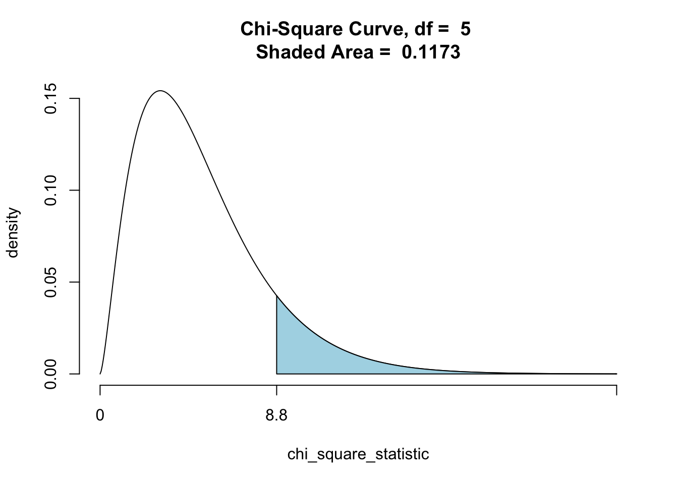
Figure 11.1: Chi-Square df=5
Since at large sample sizes the \(\chi^2\) density curve will deliver approximately the right P-value, we usually don’t ask for simulation. For the Gambler’s Die study, the function call would be:
chisqtestGC(throws,p=NullProbs)If you would like to produce a graph of the P-value, you can do so by setting the graph argument to TRUE.
chisqtestGC(throws,p=NullProbs,graph=T)If you have chose to simulate, you can get a graph of the re-sampled \(\chi^2\)-statistics:
chisqtestGC(throws,p=NullProbs,
             simulate.p.value=T,B=2500,
             graph=TRUE)
If any of the expected cell counts are below five, chisqtestGC() will issue a warning, in which case you should re-run the test using simulation.
11.3 Further Example: Seating Preference
Recalling the seating-preference variable seat in the m111survey data frame, one might ask the following
Research Qeestion: In the Georgetown College population, is there equal perference for each type of seat: front, middle and back?
In this Research Question, we are interested in the distribution of a single factor variable: seat. We can use the \(\chi^2\)-goodness of fit test to see whether the data in the m111survey provide strong evidence that the GC population is not indifferent to seat-location.
Step One: Statement of Hypotheses
If the GC population is indifferent, then the proportion of the populations that prefers each type of seat will be \(1/3\), for each of the three possible values of seat.
The Null Hypotheses may then be stated as:
\(H_0\): Each of the three types of seat is preferred by one-third of the GC population.
The Alternative disagrees:
\(H_a\): At least one of the three proportions claimed by the Null is wrong.
Step Two: Safety Check and Test Statistic
For safety, we must assume that the students in m111survey are like a simple random sample from the GC population, at least as far as seating preference is concerned.
For the test statistic and other information needed in subsequent steps, we can use formula-data input to call chisqtestGC():
chisqtestGC(~seat,data=m111survey,
            p=c(1/3,1/3,1/3))
## Chi-squared test for given probabilities
##
## Observed counts Expected by Null Contr to chisq stat
## 1_front 27 23.67 0.47
## 2_middle 32 23.67 2.93
## 3_back 12 23.67 5.75
##
##
## Chi-Square Statistic = 9.1549
## Degrees of Freedom of the table = 2
## P-Value = 0.0103We see that the P-value is about 0.01, which is less than our “cut-off” of 0.05, so we reject the Null and conclude that this data provided strong evidence that GC students are not equally likely to prefer any of the three seating locations. (The middle appears to be most desired.)
11.4 Further Example: Nexus Attendance
A Nexus event held at Georgetown College in April of the Spring semester was attended by 200 students. The class breakdown of the students is given in Table [Nexus Attendance].
| Class | Fresh | Soph | Junior | Senior |
|---|---|---|---|---|
| Freq | 62 | 27 | 33 | 80 |
Suppose that is is known that the distribution of class rank at Georgetown College is as follows:
- 30% freshmen,
- 25% sophomores,
- 25% juniors,
- 20% seniors.
We are interested in the following
Research Question: Is the attendance at April Nexus events like a random sample of GC students?
Note that in this Research Question the distribution of the variable Class Rank in the GC population in NOT at issue: everyone knows that it is given by the percentages above. What is at issue is whether the data on this Nexus event show that students are not attending randomly, in the sense that one’s likelihood of attending a Nexus event in April might be associated with one’s class rank.
In this study the hypotheses should be stated as:
\(H_0\): Attendance at the event was random.
\(H_a\): Likelihood of attendance depended on class rank.
Information needed for the remaining four steps comes from the following R-code:
Nexus <- c(fresh=62,soph=27,junior=33,senior=80)
NullClass <- c(0.30,0.25,0.25,0.20)
chisqtestGC(Nexus,p=NullClass)
## Chi-squared test for given probabilities
##
## Observed counts Expected by Null Contr to chisq stat
## fresh 62 60.6 0.03
## soph 27 50.5 10.94
## junior 33 50.5 6.06
## senior 80 40.4 38.82
##
##
## Chi-Square Statistic = 55.8482
## Degrees of Freedom of the table = 3
## P-Value = 0The \(\chi^2\) statistic was about 55.8. If the Null is true, then it should have been about 3 (the degrees of freedom), give or take
\[\sqrt{2 \times 3}=\sqrt{6} \approx 2.45\]
or so. A value of 55.8 looks very bad for the Null!
In fact, if the Null is right then the chance of getting a \(\chi^2\)-statistic of 55.8 or more is about \(4.5 \times 10^{-12}\), which is a very tiny number indeed. We reject the Null. This event provided strong evidence that, in April, Nexus attendance depends on class rank.
In fact, from the test output we see that the Null expected about 40.4 seniors to attend, whereas 80 in fact did. Apparently GC seniors are scrambling for last-minute Nexus credits!
11.5 Further Example: Too Good to be True?
Imagine that a statistics professor gives a student the following Homework assignment:
Assignment: Familiarize yourself with chance variation by rolling a fair die 6000 times. Turn in a tally of your results.
Most students would find the assignment rather onerous!
Now suppose that the next day the student hands in the results shown in Table [6000 Rolls of a Fair Die?].
| Spots | One | Two | Three | Four | Five | Six |
|---|---|---|---|---|---|---|
| Freq | 1003 | 998 | 999 | 1002 | 1001 | 997 |
The professor observes that each cell count is quite close to what would be expected in 6000 rolls of a fair die. But are the counts perhaps TOO close to what would be expected? In other words:
Research Question: Is the observed fit “too good to be true”?
Consider running a \(\chi^2\)-goodness of fit test on the data:
AllegedRolls <- c(one=1003,two=998,three=999,
            four=1002,five=1001,six=997)
FairProbs <- rep(1/6,6)
chisqtestGC(AllegedRolls,p=FairProbs)
## Chi-squared test for given probabilities
##
## Observed counts Expected by Null Contr to chisq stat
## one 1003 1000 0.01
## two 998 1000 0.00
## three 999 1000 0.00
## four 1002 1000 0.00
## five 1001 1000 0.00
## six 997 1000 0.01
##
##
## Chi-Square Statistic = 0.028
## Degrees of Freedom of the table = 5
## P-Value = 1As one might have guessed from the close agreement between observed and expected counts, the \(\chi^2\) statistic is quite small, so the P-value—the chance of getting at least this value in 6000 rolls of a fair die—is quite large: it is nearly 100%, in fact.
But think of it the other way around: if the table turned in by the student really was the result of tossing a fair die 6000 times, then what is the chance of getting such a small \(\chi^2\)-statistic? It would have to be 1 minus the P-value given in the test output:
1-0.9999931## [1] 6.9e-06This is a very small chance indeed! It would be reasonable to infer that the student made up the tally table, but did not allow for a realistic amount of chance variation away from the expected cell counts!
11.6 Thoughts About R
11.6.1 Names for Elements in a List
When you are working with summary data, you have to provide chisqtestGC() with a tally of the observed counts. The output for the test is most readable if you also provide names for each of the possible values of the factor variable under study. You can do so as you create the lists of observed counts. For example, if your variable has three possible values called “a”, “b” and “c”, with counts 13, 12 and 27 respectively, then you can create a named tally as follows:
ObsCounts <- c(a=13,b=12,c=27)11.6.2 Quick Null Probabilities
For goodness of fit tests, chisqtestGC() requires that the p argument be set to the list of proportions claimed by the Null for the factor variable under study. If these values are all the same, then you can write them quickly using the rep() function.
rep() repeats a given value a given number of times. For example to get 7 threes, just type:
rep(3,7)## [1] 3 3 3 3 3 3 3If there are eight null probabilities and they are all the same, then each would be \(1/8\), so you could set them as follows:
MyNulls <- rep(1/8,8)
MyNulls
## [1] 0.125 0.125 0.125 0.125 0.125 0.125 0.125 0.125