Chapter 6 Design of Studies

6.1 Observational Studies and Experiments

The attitudes data frame contains the results of a large-scale survey conducted at Georgetown College in the fall semester of 2001:

data(attitudes)
View(attitudes)
help(attitudes)

This dataset prompts many research questions concerning the relationship between two variables. For example, the numerical variable sentence gives the sentence recommended for a hypothetical defendant who has been convicted for involuntary manslaughter in a drunk-driving incident. Another variable—the factor major—records the type of major that the survey participant intends to pursue. A Research Question on the relationship between these two variables might take the form:

Which type of major tends to be hardest on crime?

Let’s quickly explore this question. We can take a numerical approach:

favstats(sentence~major,data=attitudes)

##        major min    Q1 median    Q3 max     mean       sd   n missing
## 1 humanities   5 11.25     20 38.75  50 25.26316 15.96565  38       0
## 2   math.sci   5 20.00     30 50.00  50 30.49351 15.64964  77       0
## 3   pre.prof   3 14.00     25 32.50  50 25.02336 15.05342 107       1
## 4 social.sci   4 15.00     25 40.00  50 25.48889 14.66694  45       0

Comparing the means of the four major groups, it seems that math and science majors recommend sentences that are, on average, about five years longer than sentences recommended by the other three major groups.

We can also take a graphical approach. Figure [Sentence by Major] also indicates that math and science majors are harder on crime. (Note, for instance, that their median is about five years above the medians for the other three groups.)

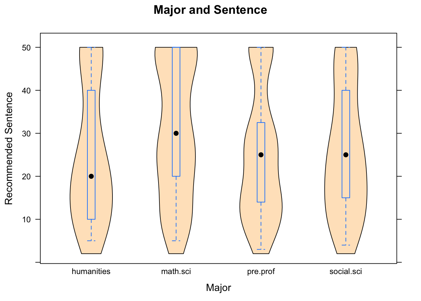
Figure 6.1: Sentence by Major. The survey respondents are broken into four groups, accordng to the type of majors they intend to pursue.

The data for this research question – the variables major and sentence – were gathered by means of an observational study:

Observational Study: In an observational study researchers simply observe or question the subjects. In particular, they measure the values of the explanatory variable $X$ and measure the values of the response variable $Y$, for each subject.

For each student in the survey, we measured the value of the variable major for each student by recording his/her choice, and observed the value of sentence by recording the sentence he/she recommended. Thus, the Research Question at hand was addressed by means of an observational study.

But not all of the variables in the attitudes data were simply observed. From the Help file on attitudes, we learn that not all subjects received the same survey form. In particular, in the question for the drunk-driving incident, some of the subjects got a form where the question was stated as follows:

You are on a jury for a manslaughter case in Lewistown, PA. The defendant has been found guilty, and in Pennsylvania it is part of the job of the jury to recommend a sentence to the judge. The facts of the case are as follows. The defendant, Tyrone Marcus Watson, a 35-year old native of Lewistown, was driving under the influence of alcohol on the evening of Tuesday July 17, 2001. At approximately 11:00 PM Watson drove through a red light, striking a pedestrian, Betsy Brockenheimer, a 20-year old resident of Lewistown. Brockenheimer was taken unconscious to the hospital and died of her injuries about one hour later. Watson did not flee the scene, nor did he resist arrest.

The prior police record for Mr. Watson is as follows: two minor traffic violations, and one previous arrest, five years ago, for DUI. No one was hurt in that incident.

Watson has now been convicted of DUI and manslaughter. The minimum jail term for this combination of offenses is two years; the maximum term is fifty years. In the blank below, write a number from 2 to 50 as your recommended length of sentence for Tyrone Marcus Watson.

Other subjects received a survey form in which the details of the incident were exactly the same as in the question above, except that the defendant’s name was given as “William Shane Winchester.” In other forms, the name of the victim varied: “Latisha Dawes”" instead of “Betsy Brockenheimer.” All told, there were four variants of the drunk-driving question:

Form-Variation in the Drunk-Driving Question
Defendant’s Suggested Race	Victim’s Suggested Race
Black	Black
Black	White
White	Black
White	White

The purpose of varying the names—and with the names, the suggested race of the person—was to investigate Research Questions like the following:

Research Question 1: Does the suggested race of the defendant have an effect on the length of sentence a subject would recommend?

Research Question 2: Does the suggested race of the victim have an effect on the length of sentence a subject would recommend for the defendant?

The data we collected for these Research Questions does not constitute an observational study: the subjects did not choose which type of form to fill out; instead the researchers (randomly) assigned forms to subjects. This makes the study an experiment.

Experiment: In an experiment, researchers manipulate something and observe the effects of the manipulation on a response variable.; Most commonly, the manipulation consists in assigning the values of an explanatory variable $X$ to the subjects.

In Research Question 1 above, the explanatory variable is defrace, the race of the defendant that is suggested by the name given to him in the form. (The response variable is sentence.) Since researchers assigned the values of defrace to each subject, Research Question 1 is being addressed through an experiment.

In Research Question 2 above, the explanatory variable is vicrace, the race of the victim that is suggested by the name given to her in the form. (The response variable is sentence.) Since researchers assigned the values of vicrace to each subject, Research Question 2 also is being addressed through an experiment.

For further practice in distinguishing between experiments and observational studies, study the following examples:

Example: Researchers test whether zinc lozenges help people with colds recover more quickly than if they took no lozenges at all. They gather 40 people who are suffering from a cold, and randomly choose 20 of them to take zinc lozenges. The remaining 20 also take a lozenge, but it the lozenge is made of an inert substance that is known to have no effect on the body.

In this situation, the explanatory variable is whether or not one takes a zinc lozenge, and the response variable is the time it takes to recover from the cold. Since researchers randomly picked who would get a zinc lozenge, the values of the explanatory variable were assigned by the researchers. This makes the study as experiment.

Example: Researchers gather a number of people. They find that, of those who wear bifocals, 5% have colon cancer. Of those who do not wear bifocals, only 1% have colon cancer.

In the second situation, the Research Question of interest appears to concern the relationship between whether or not one wears bifocals and whether or not one gets colon cancer. It’s not clear which variable—if either–is supposed to be the explanatory, but since neither variable had its values assigned to subjects (researchers did not make anyone wear bifocals, or give colon cancer to anyone!) the study is clearly just an observational study.

6.2 Why Perform Experiments?

Because in an experiment researchers assign values of the explanatory variable $X$ to subjects, experiments can be difficult to perform. For example, in the lozenge example above, most people would prefer to choose for themselves what medicine to take for a cold. In an experiment, someone else assigns the treatment to you. It’s difficult to recruit subjects for such a study!

Why, then, do researchers go to the trouble to do experiments? Why not just perform observational studies all of the time?

The answer has to do with the distinction, introduced in Chapter Four, between association and causation. We know already that two variables can be associated without there being a causal relationship between them. But there are many situations in which we really do want to know if an observed association is due to a causal relationship. Here are some examples:

We may find that smokers tend to develop lung cancer at a higher rate than non-smokers; we would like to know whether smoking actually causes lung cancer.

We may find that men drive faster than women, but we wonder whether a person’s sex is a causal factor in how fast he or she drives.

Bifocal wearers have colon cancer at a higher rate than do those who do not wear bifocals, but does this mean that wearing bifocals increases your risk of colon cancer?

Consider the last example above: we don’t think that wearing bifocals causes lung cancer, because we know that folks who wear bifocals tend to be older than those who don’t, and we know that the risk of colon cancer increases with age. Age is considered a confounding variable that explains the association between bifocal-wearing and colon cancer.

Confounding Variable: In a study with an explanatory variable $X$ and a response variable $Y$, the variable $Z$ is called a confounding variable if it meets the following three conditions:

It is a third variable (different from X and different from Y);

It is associated with X, but not caused by X.

It is a causal factor in Y (is at least part of the cause of Y)

Thus, age (Z) is indeed a confounding variable in a study of the relationship between whether or not one wears bifiocals (X) and whether or not one has colon cancer (Y). We know this because:

Age is a third variable;
Age causes bifocal wearing–older people have worse eysesight, and so choose to wear corrective lenses, including bifocals—and so age is associated with bifocal wearing.
Age helps to cause colon cancer.

Note: In Condition 2 in the definition of confounding variables we included the requirement that Z must not be caused by X. The reason for doing this is that if Z were caused by X, then, since Z helps to cause Y, X would help to cause Y indirectly after all. (We consider indirect causes to be legitimate causes; in fact, pretty much anything that we think of as a “cause” does its causal work indirectly.)

A difficulty with observational studies is that because subjects come to you with the value of their X variable already in place, observational studies are pervasively subject to the possibility of confounding variables. In the bifocal and colon cancer study, people choose whether or not to wear bifocals, and that choice is caused somewhat by their age. Hence the two groups being compared in the study—the bifocal-wearers and the non-bifocal wearers—differ with respect to age. Therefore we cannot attribute an observed difference in their colon cancer rates to the wearing of bifocals: the difference is probably due to age (or to other variables associated with age).

For another example, think back to the sat data, with which we attempted to study the relationship between teacher salary (X) and SAT score (Y) for states. Although we observed an association (states that paid their teachers more tended to have lower SAT scores), we could not conclude that paying teachers more causes their students to perform worse: the variable frac was a confounder. After all,

frac is a third variable (different from salary and from sat);
states where frac is high are states that tend to place value on education, so they are liable to pay their teachers well, so frac and salary are related;
It is likely that states with a high percentage of students taking the SAT have lower scores due to the presence in the testing pool of non-elite students, so frac helps to cause sat.

Observational studies are not rendered worthless by the mere possibility of confounding variables, but they do make things more difficult for researchers, in at least two respects:

You have to identify possible confounders BEFORE you collect your data, so you can record the value of the possible confounder for each subject in the study.
You have to figure out how to correct for the confounders.

The second requirement can be pretty tough to satisfy. One possible way to proceed is to break your data up into little groups, such that the values of the confounders are the same, or nearly the same, for the subjects in each group. That’s what we did with the sat data: recall the app:

require(manipulate)
DtrellScat(sat~salary|frac,data=sat)

The problem with breaking up the data into small subsets and studying them separately is that any relationship you see between X and Y within a subset is based on a very small sample—too small by itself to provide much evidence for a relationship in the population. Even if most of the subsets indicate the same relationship between X and Y, the fact that they were studied separately prevents us from synthesizing the results to infer a relationship between X and Y in the population at large.

Hence we would prefer to have no confounding variables in our study at all. In other words:

An Ideal: In an ideal world the different groups in the study would be exactly alike with respect to every variable that might help to cause the response variable Y, with the sole exception that the groups differ in their X-values.

For example, in the bifocal study, you would prefer to compare two groups of people that are the same with respect to:

age,
diet,
exercise patterns,
genetic history,
and anything else that might affect the risk of colon cancer!

The only way the groups would differ is that one group wears bifocals, and the other group—sometimes called the control group—does not. If two such groups were to exhibit a statistically significant difference in their colon cancer rates, then that difference could be ascribed to the bifocals, and not to anything else: there would be no confounding factors to worry about.

6.3 Experimental Designs

The ideal laid out in the preceding section cannot be attained in practice, but it can be approximated fairly well, provided that you design your experiment well.

It may surprise you to learn that good experimental designs make use of brute chance, at some point, in order to assign subjects to treatment groups. We will discuss some of these ways in this Section.

6.3.1 Completely Randomized Designs

In a completely randomized experiment, subjects are assigned to their treatment groups by randomization alone.

What is randomization, exactly, and why is it so effective in making groups similar? To see learn more about this consider again the following imaginary population:

data(imagpop)
View(imagpop)
help(imagpop)

Let’s say that the first 200 people in this population agree to be part of an experiment to see whether taking aspirin reduces the risk of heart disease.

AspHeartSubs <- imagpop[1:200,]

The experimenters plan to choose 100 of the subjects at random, and assign them to take an aspirin each morning for ten years. The remaining 100 subjects—the control group—are given a pill each morning that looks and tastes like aspirin, but has no effect on the body. (Such a substance is called a placebo, and is used to keep the subjects unaware of which group they are in. If subjects knew their group, this knowledge might determine lifestyle choices that in turn affect the risk of heart disease. When subjects in an experiment don’t know their group, the experiment is said to be single-blind.)

Together, the two groups are called the treatment groups, because they are treated differently: one groups gets aspirin, the other does not.

The X variable is whether or not the subject takes aspirin, and the Y variable is some measure of the heart-health of the subject. The values of the X variable were assigned randomly to the subjects, so this experiment has what we call a completely randomized design.

The R-function RandomExp() carries out the randomization:

Assignment <- RandomExp(AspHeartSubs,
                  sizes=c(100,100),
                  groups=c("placebo","aspirin"))

You should take a look at the result:

View(Assignment)

As you can see, 100 of the subjects are assigned to the Placebo group, and the other 100 are assigned to the Aspirin group. The assignment is done at random: each subject was equally likely to be assigned to either group.

Recall that we would like the treatment groups to be similar in every way, except that one group takes aspirin and the other does not. In order to verify that they are reasonably similar, we can check to see whether the variable treat.grp is related to any of the other variables in the Assignment data frame.

Do the treatment groups differ much with respect to sex (i.e., is treat.grp related to sex)? Let’s see:

SexGrp <- xtabs(~treat.grp+sex,data=Assignment)
rowPerc(SexGrp)

##          sex
## treat.grp female male Total
##   placebo     51   49   100
##   aspirin     56   44   100

The distribution of sex in the two treatment groups appears to be quite similar.

Do the groups differ much with respect to income? (Is treat.grp related to income?) Let’s see:

favstats(income~treat.grp,data=Assignment)

##   treat.grp  min    Q1 median    Q3    max  mean       sd   n missing
## 1   placebo 1200 18325  33600 50000 154700 39215 26995.24 100       0
## 2   aspirin 1500 16675  33550 55650 165700 39486 29352.24 100       0

The means and medians of the two groups appear to be quite similar.

For further practice, pick another variable in the Assignment data frame, and see if the treatment groups differ much with respect to that variable.

The randomization procedure is not perfect: if you repeat the procedure many times:

Assignment <- RandomExp(AspHeartSubs,
                sizes=c(100,100),
                groups=c("placebo","aspirin"))

From time to time you will discover that for one or two of the variables the treatment groups are somewhat different. But on the whole it appears likely that for the most part the treatment groups will be pretty similar.

When R was doing the randomization to create the treat.grp variable, it worked “blindly”: it did not take into account the sex, income, etc. of any of the subjects. This means that when researchers adopt a completely randomized design, they don’t have to keep track of any characteristics of their subjects – not even those characteristics that might be confounding factors. Blind chance by itself is likely to produce similar treatment groups.

Statistical theory tells us that, the larger the number of subjects, the more likely it is that the treatment groups will be similar, and the more similar they are likely to be! That’s one reason why researchers like to get as many subjects as possible into each treatment group. This principle is called replication:

Replication: An experiment is said to involve replication if each the treatment group contains more than one subject. (The more subjects there are in each group, the more replication the experiment has.)

6.3.2 Randomized Block Designs

6.3.2.1 Dealing with a Small Number of Subjects

So far we have looked at experiments with a completely randomized design. This design works very well when you have a lot of subjects, because then you can get a lot of subjects into each treatment group. Blind chance then guarantees—more or less—that the treatment groups will be similar. When you don’t have a lot of subjects, however, things might not go so well.

Suppose, for example, that you want to do an experiment to compare two weight-lifting programs (Program A and Program B), to see which one is more effective. You have 16 subjects in your group:

data(SmallExp)
View(SmallExp)
help(SmallExp)

Note that the sex and athletic status (athlete or not) of each subject has been recorded.

Your plan is to break the subjects into two groups of size 8 each. Group A will train with Program A for ten weeks, and Group B will train with Program B. At the end of the ten-week period, you will measure the increase in strength for each subject.

Let’s say you decide on a completely randomized design:

RandomExp(SmallExp,sizes=c(8,8),
          groups=c("Program.A","Program.B"))

Perform the randomization several times by re-running the above code. Are you always happy with the results, or do the treatment groups often look rather different with respect to sex and/or with respect to athletic status?

When the number of subjects is small, randomization can easily produce dis-similar treatment groups. If the treatment groups are dis-similar with respect to possible confounders (such as Sex and athlete in this study) then we have a problem.

6.3.2.2 Blocking

Accordingly, when an experiment is expected to have only a small number of subjects, researchers will often adopt a randomized block design. This means that they carry out the following procedure:

For each subject, record the values of variables that you consider to be potential confounders. In the current study, sex and athlete have been recorded.
Break the subjects into blocks based on combinations of values of the potential confounders. In this study the blocks would be:
- the four females who are athletes
- the four females who are not athletes
- the four males who are athletes
- the four males who are not athletes
Within each block randomly assign subjects to treatment groups. In this study, for example, you would randomly pick two of the female athletes to be in Group A, with the other two going to Group B, and do the same for the other three blocks.

Randomized blocking is accomplished with RandomExp() as follows:

RandomExp(SmallExp,sizes=c(8,8),
          groups=c("Program.A","Program.B"),
          block=c("sex","athlete"))

Re-run the randomization several times, and observe that:

In terms of the individuals, the treatment groups differ from one run to another.
But they are the same every time, as far as the values of sex and athlete are concerned.

The basic idea of blocking is to ensure that—at least with respect to a few variables whose values you can record in advance—the two groups will be similar. Naturally, the variables for which you would choose to block should be variables that are strongly associated with the response variable. If you block for them, then the treatment groups are the same with respect to these variables and you will have reduced the number of confounding variables you need to worry about.

As an example of a randomized block design, consider the saltmarsh data frame:

data(saltmarsh)
View(saltmarsh)
help(saltmarsh)

The data frame contains the results of an experiment to study the effects of salinity levels in soil on the growth of plants. Researchers had access to four different fields of equal size at an agricultural research station. They divided each field into six plots of equal size and treated each plot with one of six concentrations of salt, ranging from 10 to 35 parts per million. They allowed plants to grow on the fields for a period of time, and then measured the total biomass of each plot.

In this experiment the subjects are the plots—24 of them, all told, six in each field. The explanatory variable is the salinity level salt, and the response variable is biomass. Since the four fields probably contained different types of soil and were subject to differing environmental conditions, the field to which a plot belongs could have a considerable effect on plant growth: hence it was considered important to block for “field”, and so each field was subdivided into six equal plots. Within each field, the six levels of salinity were assigned randomly to the six plots in that field. In the data frame, the field-variable is recorded as block.

You can check directly that blocking was indeed performed:

xtabs(~salt+block,data=saltmarsh)

##     block
## salt Field1 Field2 Field3 Field4
##   10      1      1      1      1
##   15      1      1      1      1
##   20      1      1      1      1
##   25      1      1      1      1
##   30      1      1      1      1
##   35      1      1      1      1

Sure enough: the six treatments groups (the salt levels) are distributed identically with respect to block.

In order to address the Research Question, we note that the explanatory and response variables are both numerical, so a scatterplot could be an appropriate graphical tool. Figure [Biomass and Salinity] shows the scatterplot, and indeed it does appear that there is a negative relationship between salinity-level and biomass.

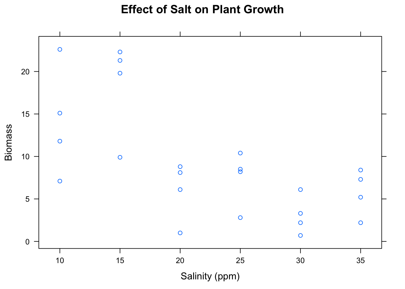
Figure 6.2: Biomass and Salinity. The higher the concentration of salt, the lower the biomass in the plot.

6.3.3 Matched Pair Designs

A matched pair design is really an extreme form of blocking.

Suppose that you want to form two treatment groups: Group A and Group B. You pair up your subjects so that the members of each pair are as similar as possible to one another. Each pair is a considered to be a “block.” Then for each pair, one member is assigned randomly to Group A, and the other is assigned to Group B.

Here is a well-known example of a matched pair design. Suppose you want to see which type of shoe sole, type A or type B, wears out more quickly, and say that you have 20 people who agree to participate in your experiment. Each person has a pair of feet, and these forty feet constitute the “subjects” in the experiment. The two members of any given pair of feet are pretty similar with respect how much wear they will put on a shoe—after all, both members of the pair belong to the same person, and hence are engaged in pretty nearly the same set of daily activities—so you randomly assign 10 of the subjects to wear a type-A sole on their left foot and a type-B sole on their right foot. The other ten will do the reverse. In this way, the members of each pair of feet has been assigned randomly to one of the treatment groups! (Randomization is especially important here, because most people tend to favor one foot over the other.)

6.3.4 Repeated-Measure Designs

For the purposes of this course, an experiment is said to employ a repeated-measure design if the researchers make two or more similar measurements on each individual in the study, with a view to studying the differences between these measures.

As an example, consider the data frame labels:

data(labels)
View(labels)
help(labels)

The labels data frame contains the results of an experiment conducted at Georgetown College by two students. The students wanted to investigate whether one’s belief about the price of a brand item would, in and of itself, affect one’s perception of its quality. Thirty fellow students served as subjects. One at a time, each subject was brought into a room where two jars of peanut butter were placed on a table. One jar had the well-known “Jiff” label, and the other had the Great Value label. (Great Value is the Wal-Mart brand, and is considered “cheaper.”) The subject tasted each peanut butter and rated it on a scale of 1 to 10. Unknown to the subjects, both jars contained the exactly the same peanut butter: the Great Value brand.

In this experiment, the two similar measurements are the rating given to the jar of peanut butter that is labeled Jiff, and the rating given to the jar labeled Great Value. What makes this repeated-measures study an experiment is not that researchers assigned the values of some explanatory variable to subjects, but rather that they manipulated the situation so the subjects believed that the experiment was a taste test to compare two different types of peanut butter, when it fact it was designed to compare their reactions to different labels on the SAME peanut butter.

(Note: Some people like to say that every experiment involves assigning the values of the X variable to subjects. Such persons would maintain that in this experiment, the X variable is the kind of label (Jiff or Great Value), and that the experimenters were able to assign BOTH values of X to each subject. When you think about it this way, the two treatment groups are quite similar indeed, because they are composed of exactly the same set of subjects!)

When measures are repeated, there is always the possibility that the second measurement might depend in some way on the first. In this case, the rating given to the peanut butter in the second jar tasted might be affected by the fact that the subject has recently tasted some peanut butter (from the first jar). In order to wipe out the effects of any such dependence, it is good practice to randomly vary the order in which the measurements are made. In this experiment, for example, you might determine in advance for each subject—by coin toss perhaps—whether he or she is to taste from the Jiff-labeled jar first or from the Great Value-labeled jar first. (It is also good practice to record the order of tasting, though unfortunately the researchers did not do this.)

We would like to see whether subjects tended to rate the jar labeled with the more expensive brand as more highly, on the whole, so we are interested in the difference of the repeated measures

diff <- labels$jiffrating - labels$greatvaluerating

We can look at the difference in a variety of ways. Numerically:

favstats(~diff)

##  min Q1 median Q3 max     mean       sd  n missing
##   -5  1    2.5  4   8 2.366667 2.809876 30       0

We see that the subjects rated the Jiff-labeled peanut butter an average of 2.37 points higher than they rated the peanut butter from the Great-Value-labeled jar. A graphical approach is shown in Figure [Ratings Difference].

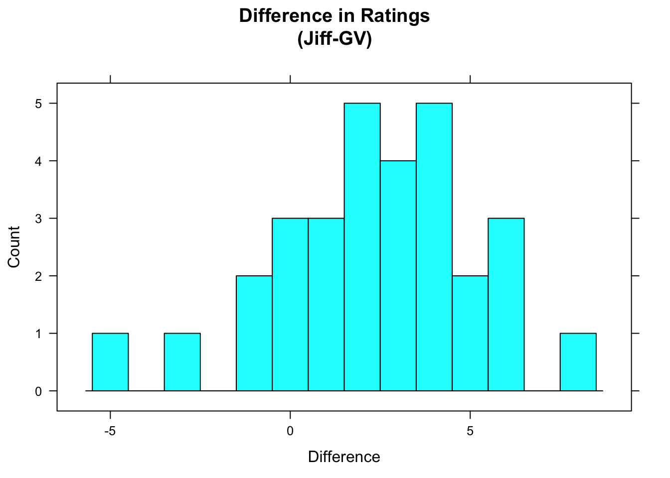
Ratings Difference. Most of the differences are positive, indicating that subjects usually rated the Jiff-labeled peanut butter more highly.

Figure 6.3: Ratings Difference. Most of the differences are positive, indicating that subjects usually rated the Jiff-labeled peanut butter more highly.

A repeated-measures design appears to be the gold-standard among experiments, since your treatment groups are – in some sense – the same group. But is it always feasible to perform a repeated-measures experiment?

Consider, for example, the following (thankfully hypothetical) Knife-or-Gun study:

data(knifeorgunblock)
View(knifeorgunblock)
help(knifeorgunblock))

The Research Question was:

What will make you yell louder: being killed with a knife or being killed with a gun?

Would it have been feasible to perform this experiment with a repeated measures design? Probably not: once a subject is slain by one method, be it Knife or Gun, he/she probably will make no noise at all whilst being subjected to the subsequent method of slaying! As a result, we would have only one useful measurement on each subject.

On a more serious note:

Consider the attitudes study, in which a completely randomized design was employed. Suppose we had tried to run the study as a repeated measures experiment, giving each subject all of the different kinds of form, perhaps in some random order determined by a coin toss: what would have happened? Would the repeated-measures design have been any improvement over a completely randomized design?

6.4 Considerations About Experiments

6.4.1 Reproducibility

When you do any sort of scientific work, you want your results to be reproducible as much as possible, so that others may see exactly how you obtained these results, and thereby check them. Accordingly, when you are actually doing an experiment, even your randomization needs to be done in such a way that another person could reproduce it entirely. In R this is accomplished by the set.seed() function.

Consider the following small block of code:

set.seed(314159)
RandomExp(SmallExp,sizes=c(8,8),
          groups=c("Program.A","Program.B"),
          blocks=c("sex","athlete"))

You will recognize the call to RandomExp() as the same call you performed earlier in the chapter, in order to randomize subjects into treatment groups after blocking for sex and athlete. This time, however, the call to RandomExp() is preceded by a call to set.seed(). This call “starts out” the randomization from a fixed point in R—called a seed—so that no matter how many times you run the above code chunk you will get the same results each time.

The seed is the integer that is supplied to the set.seed() function. This time, the seed was 314159: the first few digits of the number $\pi$. In general, you should choose a seed that stands for something familiar, so that others who examine your code can see that you did not just keep on trying out different seeds until you got the sort of results you wanted.

6.4.2 Subjects and the Population

So far we have highlighted a major advantage of experiments over observational studies, namely that in an experiment you have the opportunity to reduce or eliminate the effect of confounding factors by the appropriate use of such techniques as randomization, blocking, matched pairs, and so on.

However, researchers wishing to perform experiments on human subjects face a problem that does not crop up—at least not in such an extreme form—in the course of conducting an observational study. The problem is one of consent.

You can’t just compel people do one thing or another. You can’t grab people at random off the street and assign a value of an explanatory variable to them:

“Hey, you, there! Yes, you! Come over here! You are hereby inducted into my experiment. Um, wait a minute while I flip this coin. OK, it’s settled: you will ____ [insert smoke if toss was heads, not smoke if toss was Tails] for the next twenty years! Got it?”

Since people must consent to be in an experiment, the set of people who are willing to be in the experiment may be quite different from the population at large. It is well known, for instance, that people who volunteer for medical experiments tend to be more educated and to have higher incomes than those who refuse to participate in such experiments. Anyone who would consent to be part of the Knife or Gun experiment (see the previous section) would have to be stark raving mad—surely that makes them different from the general population.

In general:

If the subjects differ from the general population in ways that are associated with how they respond to the different treatments available in the experiment, then the results of the experiment can at most be said to apply to the subjects themselves.

In such a case we must exercise a great deal of caution when applying our results to some larger population.

6.4.3 Statistical Significance

Even when the subjects are quite different from the population, and we are reduced to wondering whether the the treatments made a difference for those subjects only, statistical significance is still an issue. Consider once again the Knife or Gun experiment.

Who did yell louder, in the experiment: the subjects who were killed by knife, or the subjects who were killed by gun? Let’s see:

favstats(volume~means,data=knifeorgunblock)

##   means  min     Q1 median     Q3  max  mean        sd  n missing
## 1   gun 40.3 45.925  53.25 59.925 64.5 53.00  8.761152 10       0
## 2 knife 61.2 65.200  72.00 77.125 90.9 73.13 10.071528 10       0

A nice graphical tool for small data sets is a strip plot, which we combine here with a violin plot (see Figure [Knife or Gun?]):

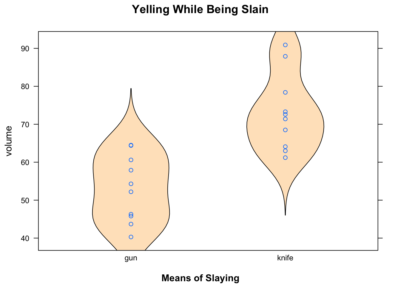
Figure 6.4: Knife or Gun? Apparently those slain by Knife yell louder!

Hmm, it appears the subjects who were slain by knife yelled louder: the volume-points, and their violin, is somewhat higher than the points and violin for those slain by a gun.

But are the results statistically significant? By this question we do NOT mean:

“Could the difference reasonably be ascribed to chance variation in the process of sampling subjects from the population?”

These subjects aren’t a random sample from the population at all. Maybe they were the ONLY 20 people in the world who would agree to be part of the experiment, so there was no chance at all involved in their selection.

Instead, the question of statistical significance addresses the randomness that was at play in the experiment: namely, the random assignment of subjects to Knife or Gun group.

So we are REALLY asking:

“Is the observed difference in dying screams due to the means of slaying, or is is reasonable to believe that in the random process of assigning subjects to groups, a lot of naturally loud yellers just happened to get into the Knife group?”

In any experiment where randomization was employed, the question of statistical significance is meaningful, and it can always be thought of as asking:

“Do the results indicate that X causes Y, or is reasonable to ascribe the observed difference between the treatment groups to chance variation in the assignment of the subjects to their groups?”

See the GeekNotes for some preliminary assessment of statistical significance in some of the experiments discussed in this chapter.

6.5 Terminology for Experiments

Here follows a list of technical terms, associated with experiments and observational studies, that we would like you to know. If a term has already been introduced, then it is simply listed below with its definition. If it has not been discussed yet, then we offer a brief explanation and/or examples.

Observational Study: In an observational study researchers simply observe or question the subjects. In particular, they measure the values of the explanatory variable $X$ and measure the values of the response variable $Y$, for each subject.
Experiment: In an experiment researchers manipulate something and observe the effects of the manipulation on a response variable.; Most commonly, the manipulation consists in assigning the values of an explanatory variable of $X$ to the subjects.
Confounding Variable: In a study with an explanatory variable $X$ and a response variable $Y$, the variable $Z$ is called a confounding variable if it meets the following three conditions:

It is a third variable (different from X and different from Y);

It is associated with X, but not caused by X.

It is a causal factor in Y (is at least part of the cause of Y)

Experimental Units: The experimental units (also called the individuals) are the subjects in an experiment.

Subjects do not have to be human beings, or animals. Recall, for example, the matched-pair shoe experiment in which the subjects were the 40 feet of the twenty human participants!

Treatment Groups: The treatment groups of an experiment are the groups into which the subjects are divided.
Control Group: If one group in an experiment is not treated in any special way, or is present for comparative purposes, then this group is often called the control group.
Single-Blind Experiment: If the subjects in an experiment do not know which treatment group they are in, then the experiment is said to be sinble-blinded.; If the people who measure the response variable do not know which groups the subjects are in, then the experiment is also-said to be single-blinded.
Placebo: A placebo is an inert substance given to subjects in the control group. It resembles the substances given to subjects in the other treatment groups, and thus allows the experiment to be single-blinded.
Double-Blinded Experiment: If neither the subjects nor the people responsible for measuring the response variable know the group assignments of the subjects, then the experiment is said to be double-blinded.

Blinding is useful as a means of reducing bias. If subjects know their treatment group, then this knowledge can affect their behavior in ways that have a bearing on the response variable. For example, in a study on the effectiveness of a vaccine against a particular diseases, subjects who know they are receiving the vaccine may behave more recklessly than subjects who know that they are in a control group (not receiving any vaccine). These differences in behavior could bias the study against the vaccine.

The people who are responsible for measuring the response variable could “skew” the measurements in one direction or another, if they have some stake in the outcome of the experiment. Keeping these researchers in the dark as to the group assignment of subjects with whom they work can reduce bias that arises from a desire to have the experiment “succeed”.

Replication: An experiment is said to involve replication if each the treatment group contains more than one subject. (The more subjects there are in each group, the more replication the experiment has.)
Double-Dummy Design: A double-dummy design is a procedure to blind an experiment, even when the treatments don’t resemble each other at all.

A classic example of a double-dummy design is an experiment to compare two methods of delivering nicotine to the bodies of people who desire two quit smoking. One method involves wearing a patch that delivers nicotine through the skin, and the other involves chewing gum that contains nicotine. In a double-dummy experiment:

Members of the Patch Group wear a real nicotine patch, and chew a gum that looks and tastes like real nicotine gum but which actually contains no nicotine;
Members of the Gum Group chew real nicotine gum, and wear a patch that looks the same as a nicotine patch but which delivers no nicotine.

In neither group would subjects be able to tell which group – Patch or Gum – they are in.

6.6 Thoughts on R

6.6.1 New R-functions

Just one new R-function to learn: RandomExp(), for completely randomized designs and for blocking. Here are some examples of its use. Suppose you have a data frame called MyData, that contains the list of subjects, and possibly some other variables of interest for which you might like to block.

For a completely randomized design into two groups with groups sizes $n_1$ and $n_2$, with group names “Group.A” and “Group.B”, use:

RandomExp(MyData,sizes=c(n1,n2),
          groups=c("Group.A","Group.B")

For three groups (“Group.1”, “Group.2” and “Group.3”) with sizes $n_1$, $n_2$ and $n_3$, blocking with respect to the variable Var, use:

RandomExp(MyData,sizes=c(n1,n2,n3),
    groups=c("Group.1","Group.2","Group.3"),
    block="Var")

To block for two variables Var1 and Var2 at once, use:

RandomExp(MyData,sizes=c(n1,n2,n3),
    groups=c("Group.1","Group.2","Group.3"),
    block=c("Var1","Var2"))

Make sure that the group sizes sum to the number of rows in the data frame, and that the blocking variables are factors.

6.6.2 “Book-Chapter” Notation

Sometimes you have to manipulate variables in a data frame directly, outside of the context of a function that takes formula-data input. In such a case, you can use what we call “book-and-chapter” notation to help R locate the variables of interest.

If variable Var is in data frame MyData, then R can locate it if you use a $-sign and write it as:

Mydata$Var

For example, to compute the difference of two variables in MyData, you could use:

diff <- MyData$Var1 - MyData$Var2

The data frame MyData is like a book, and the $-sign instructs R to look inside the “book” MyData at “chapters” Var1 and Var2.