10  Basic Tidyverse Concepts

The Treachery of Images (Rene Magritte, 1948).

In this chapter we will introduce:

• the pipe-operator |> that is used to chain function-calls in an inutitive, readable way;
• a few tools from the tidyverse set of R-packages, including:
  • the tibble class, a variant of the data frame that is especially suitable for large data sets;
  • data manipulation functions from the dplyr package suitable for use with data tables the pipe operator:
    • filter() and select() for sub-setting a table;
    • mutate() for transforming variables in a table;
    • summarise() for numerical summaries;
    • arrange() to rearrange the rows of a table according to the alphabetical or numerical order of one or more of its columns.

10.1 The Tidyverse

The tidyverse isn’t a package, exactly—it’s a collection of packages. Go ahead and attach it:

library(tidyverse)

You’ll get an account of the packages that have been attached. We have worked before with ggplot and by the end of CSC 215 we will have worked with all of the others. You need not worry about the fact that filter() and lag() mask functions from the stats package.

10.2 The Pipe Operator

The pipe operator, |> connects two function calls by making the value returned by the first call the first argument of the second call. Here’s an example:

"hello" |> rep(times = 4)

[1] "hello" "hello" "hello" "hello"

This is the same as the more familiar:

rep("hello", times = 4)

[1] "hello" "hello" "hello" "hello"

Here’s another example:

# same as nrow(bcscr::m111survey)
bcscr::m111survey |> nrow()

[1] 71

Here’s two pipes:

"hello" |> rep(times = 4) |> length()

[1] 4

By default the value of the left-hand call is piped into the right-hand call as the first argument. You can make it some other argument using the underscore _ as a placeholder, for example:

4 |> rep("hello", times = _)

[1] "hello" "hello" "hello" "hello"

Caution 10.1: Piping Past the First Argument

If you plan to make the result of left-hand side of the |> act as the second or subsequent argument for the function on the right-hand side, tha argument must have a paramter anem and you must use it.

For example, this works:

4 |> rep("hello", times = _)

[1] "hello" "hello" "hello" "hello"

But this won’t work:

4 |> rep("hello", _)

Error in rep("hello", "_"): pipe placeholder can only be used as a named argument (<input>:1:6)

When the arguments don’t have names, you are out of luck. For example, suppose you want to cat out “Hello there”, using |>. This would work:

"Hello" |> cat("there")

Hello there

But you cannot start with “there”:

"there" |> cat("hello", _)

Error in cat("hello", "_"): pipe placeholder can only be used as a named argument (<input>:1:12)

There is no way to fix this, because cat() does not have parameter-names for the arguments that it plans to stick together.

Since sub-setting is actually a function call under the hood (look ahead to Section 14.2.1), you can use the underscore there, too:

# gets the third element of the sequence 1, 4, 9, ..., 97:
seq(1, 100, by = 4) |> _[3]

[1] 9

Similarly, since the $-operator that we use access elements of objects such as data frames and lists is also a function (see again Section 14.2.1), you can do things like this:

# access height in m111survey:
bcscr::m111survey |> _$height

The pipe operator isn’t all that useful when you only use it once or twice in succession. Its true value becomes apparent in the chaining together of many manipulations involving data frames.

10.2.1 Practice Exercises

Tip 10.1: Rewriting with the Pipe

Problem

Rewrite the following call with the tidyverse pipe operator, in three different ways:

Solution

Note that in the second expression, we actually had to provide the name of the to parameter, in accordance with Caution 10.1.

Tip 10.2: More Rewriting with the Pipe

Problem

Use the pipe operator with subset() to find the row of mosaicData::CPS85 containing the worker who made more than 40 dollars per hour. Display only the sex, age and wage of the worker.

Solution

10.3 Tibbles

The tibble package gives us tibbles, which are very nearly the same thing as a data frame. Indeed, the name “tibble” is supposed to remind us of a data “table.”

Consider the class of bcscr::m111survey (see Data Table 7.1):

class(bcscr::m111survey)

[1] "data.frame"

Yep, it’s a data frame. But we can convert it to a tibble, as follows:

survey <- as_tibble(bcscr::m111survey)
class(survey)

[1] "tbl_df"     "tbl"        "data.frame"

You can treat tibbles like data frames. For now the primary practical difference is manifest when you print a tibble to the Console:

The output is automatically truncated, and the number of columns printed is determined by the width of your screen. This is a great convenience when one is dealing with larger data sets.

Many larger data tables in packages will come to you as tibbles.

10.4 Subsetting with dplyr

The dplyr function filter() is the rough equivalent of select(): it picks out rows of a data frame (or similar objects such as a tibble). The dplyr function select() subsets for columns.

Thus you can use the two functions together to do perform sub-setting. With the pipe operator, your code can be quite easy to read:

Note that dplyr data-functions like filter() and select() take a data table as their first argument, and return a data table as well. Hence they may be chained together as we saw in the above example.

With select() it’s easy to leave out columns, too:

10.4.1 Practice Exercises

Tip 10.3: Subsetting with the Pipe

Problem

Can you use the pipe to chain dplyr functions along with nrow() to find out how many people in survey believe in love at first sight and drove more than 120 miles per hour?

Solution

Tip 10.4: More Subsetting with the Pipe

Problem

In survey, find the three largest heights of the males who drove more than 120 miles per hour.

Solution

This is one way, using functions you already know:

Tip 10.5: CPS85 Wages

Problem

Use the pipe and filter() to make violin plots of the wages of men and women in CPS85 (see Data Table 7.3), where the outlier-person (whose wage was more than 40 dollars per hour) has been eliminated prior to making the graph.

Solution

Tip 10.6: Naming Your Child “Leslie”

Problem

The babynames package has a data table called babynames (see Data Table 10.2):

babynames

# A tibble: 1,924,665 × 5
    year sex   name          n   prop
   <dbl> <chr> <chr>     <int>  <dbl>
 1  1880 F     Mary       7065 0.0724
 2  1880 F     Anna       2604 0.0267
 3  1880 F     Emma       2003 0.0205
 4  1880 F     Elizabeth  1939 0.0199
 5  1880 F     Minnie     1746 0.0179
 6  1880 F     Margaret   1578 0.0162
 7  1880 F     Ida        1472 0.0151
 8  1880 F     Alice      1414 0.0145
 9  1880 F     Bertha     1320 0.0135
10  1880 F     Sarah      1288 0.0132
# ℹ 1,924,655 more rows

Each row is the set of babies born in U.S. hospitals in the given year who were of the stated sex and had the stated name. In addition, the table gives:

• n: the number of babies in the group;
• prop: the proportion of all babies of the stated sex who had the stated name.

Use babynames to investigate the relative popularity of Leslie as a name for boys vs. a name for girls, over the years. You should make a graph like this:

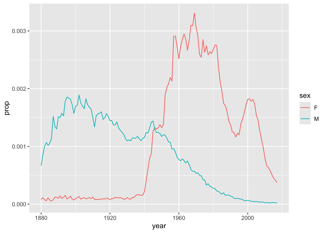
Hint: The line-graphs are made with geom_line().

Solution

10.5 Transforming Variables with dplyr

In dplyr you transform variables with the function mutate(). Here is an example:

In mutate() there is always a variable-name on the left-hand side of the = sign. It could be the same as an existing variable in the table if you are content to overwrite that variable. On the right side of the = is a function that can depend on variables in the data table.

You can transform more than one variable in a single call to mutate(), as in the code below. Try it!

10.5.1 Practice Exercises

Tip 10.7: Transforming Variables

Problem

In mosaicData::CPS85 (see Data Table 7.3) transform the wage variable to units of dollars per day. (Assume an 8-hour working day.). Show only the first 10 rows.

Solution

10.6 Summarizing, Grouping, and Rearranging

The next dplyr data-function, summarize(), is useful for generating numerical summaries of data.

Consider, for example, CPS85 (see Data Table 7.3), and suppose that you want to find the mean wage of all the workers. We can get it with summarize()

You can get multiple numerical summaries with just once call to summarize():

We know from graphical studies that the men in the study are paid more than women, but how might we verify this fact numerically? One approach would be to separate the men and the women into two different groups and compute the mean wage for each group. summarise() can do this for us, if we make use of its .by parameter:

Of course you can still create more than one summary:

In the previous example, dplyr::n() was used to count the number of cases in each group.

For a more complete account of a numerical variable, one might consider the five-number summary:

• the minimum value
• the first quartile (Q1)
• the median
• the third quartile (Q3)
• the maximum value

These quantities are conveniently computed by R’s fivenum() function:

CPS85 |> 
  _$wage |> 
  fivenum()

[1]  1.00  5.25  7.78 11.25 44.50

Let’s find the five number summaries for the wages of men and women:

It’s also possible to group by more than one variable at a time. For example, suppose that we wish to compare the wages of men and women in the various sectors of employment. All we need to do is group by both sex and sector:

Note that there were no women in the construction sector, so that group did not appear in the summary.

But the table isn’t easy to use! If we aim to compare wages of women and men within each sector, we would rather see the rows arranged like this:

     sector sex  n  min    Q1 median     Q3   max
1  clerical   F 76 3.00 5.100  7.000  9.550 15.03
2  clerical   M 21 3.35 6.000  7.690  9.000 12.00
3     const   M 20 3.75 7.150  9.750 11.825 15.00
4     manag   F 21 3.64 6.880 10.000 11.250 44.50
5     manag   M 34 1.00 8.800 13.990 18.160 26.29
6     manuf   F 24 3.00 4.360  4.900  6.050 18.50
7     manuf   M 44 3.35 6.585  8.945 11.250 22.20
8     other   F  6 3.75 4.000  5.625  6.880  8.93
9     other   M 62 2.85 5.250  7.500 11.250 26.00
10     prof   F 52 4.35 7.025 10.000 12.275 24.98
11     prof   M 53 5.00 8.000 12.000 16.420 24.98
12    sales   F 17 3.35 3.800  4.550  5.650 14.29
13    sales   M 21 3.50 5.560  9.420 12.500 19.98
14  service   F 49 1.75 3.750  5.000  8.000 13.12
15  service   M 34 2.01 4.150  5.890  8.750 25.00

For this, we use dplyr’s arrange() function:

arrange() puts the rows in order of the values of the columns it is given. In the application above it arranges the rows in alphabetical order of the sectors, and within each sector the rows are arranged in alphabetical order of sex.

10.6.1 Note on Binding

Keep in mind that you can always “save” the results of any computation by binding them to a variable name, thus:

As you can see, the result is just another data.frame, so you may work with it in any of the ways you have learned. You could do further manipulation with dplyr functions, you could make a plot—whatever you like.

10.6.2 Practice Exercises

These exercises deal with the flights data table from the nycflights13 package.

Dataflights Info

Description

 On-time data for all flights that departed NYC (i.e. JFK, LGA or EWR)
 in 2013.

Format

 Data frame with columns
 
 year, month, day Date of departure.
 
 dep_time, arr_time Actual departure and arrival times (format HHMM or
           HMM), local tz.
 
 sched_dep_time, sched_arr_time Scheduled departure and arrival times
           (format HHMM or HMM), local tz.
 
 dep_delay, arr_delay Departure and arrival delays, in minutes. Negative
           times represent early departures/arrivals.
 
 carrier Two letter carrier abbreviation. See 'airlines' to get name.
 
 flight Flight number.
 
 tailnum Plane tail number. See 'planes' for additional metadata.
 
 origin, dest Origin and destination. See 'airports' for additional
           metadata.
 
 air_time Amount of time spent in the air, in minutes.
 
 distance Distance between airports, in miles.
 
 hour, minute Time of scheduled departure broken into hour and minutes.
 
 time_hour Scheduled date and hour of the flight as a 'POSIXct' date.
           Along with 'origin', can be used to join flights data to
           'weather' data.

View

Data Table 10.1

Tip 10.8: Flights: Departures and Delay

Problem

The flights table gives information about each departure in the year 2013 from one of the three major airports near New York City: John F. Kennedy (JFK), LaGuardia (LGA) or Newark (EWR).

• The airport from which the plane departed is recorded in the variable origin.
• The variable dep_delay gives the delay in departure, in minutes. (This is a negative number if the plane left early).

Find the number of departures and the mean departure delay for each of the three airports. (Note that dep_delay for cancelled flights will be NA.)

Solution

Tip 10.9: Flights: Distance Travelled

Problem

• The variable distance gives the distance, in miles, between an origin and destination airport.
• month gives the number of the month when the flight was scheduled (1 = January, etc.).
• day gives the day of the month the flight was scheduled.

For July 26, 2013, make a violin plot of the distances traveled by the departing planes from the each of the three New York airports. Use the pipe and filter() to take flights into the desired plot.

Solution

Tip 10.10: Flights: a Long, Long Way

Problem

Examine the plot you made in the previous problem: two of the flights appear to be about 5000 miles. Use the pipe, filter() and select() to display the origin, destination and distance for these two flights.

Solution

Try this:

Tip 10.11: Short Flights

Problem

Make a table that shows the ten shortest flights in increasing order of the distance travelled from the origin to the destination. Show only the columns for the flight number, the origin, the destination, and the distance.

Hint: Apply arrange() and then head().

Solution

Try this:

Wow: there is a flight that goes from one NYC airport to another.

Tip 10.12: Long Flights

Problem

Make a table that shows the ten longest flights in decreasing order of the distance travelled from the origin to the destination. Show only the columns for the flight number, the origin, the destination, and the distance.

Hint: Read the Help for the dplr function desc():

Solution

Try this:

Flight 51 goes all the way to Honolulu!

10.7 The Tidyverse Pipe

The first pipe in R was actually made available by the magrittr package. It is symbolized by %>%. This pipe was incorporated into the tidyverse tools and became so popular that the R Core Team decided to write a pipe operator for R’s base package: that’s the |>. Since it’s in package base that is always attached when an R session begins, |> is called the “native” pipe for R.

The native pipe has since become very popular. But you’ll see the %>% quite a bit, perhaps even later on in this textbook, so let’s take a quick look at how it works.

For our purposes, %>% R’s can be used interchangeably with |>, except that the placeholder is indicated by the dot (.) instead of an underscore.

A few examples:

Note 10.1: %>% is Less Uptight

Another difference between %>% and |> is that, in contrast to Caution 10.1, %>% allows you to pipe the result of the left-hand side into the second or subsequent argument of the right-hand side, even when that argument is not named. For example, this works:

4 %>% rep("hello", .)

[1] "hello" "hello" "hello" "hello"

So does this:

"there" %>% cat("hello", .)

hello there

Tip

At the time of writing this tip, the R Studio keyboard shortcut:

• Ctrl+Shift+M on Windows/Linux, or
• Cmd+Shift+M on Mac OS

is currently set to produce %>%, but it can be made into a shortcut for |>, if you like. To set this up in R Studio:

• Open the Tools menu.
• In the Tools menu, select Global Options.
• On the sidebar of the resulting dialog box, pick Code.
• Check for box for “Use native pipe operator”.
• Press the Apply button at the bottom.

Links to Class Slides

Quarto Presentations that I sometimes use in class:

• All Sections
• Extra Practice with babynames

Exercises

Exercise 1

Use the pipe operator to rewrite the following command in three ways:

runif(10, min = 0, max = 5)

Hint: Review Practice 10.1.

Exercise 2

Rewrite the following command using two pipe operators in succession:

paste("hello", "there", "Bella")

[1] "hello there Bella"

Exercise 3

Use the pipe operator and dplyr functions to rewrite the following command:

head(subset(m111survey, sex == "female")[, c("height", "fastest")], 6)

Exercise 4

This and the next exercise are about the babynames data frame from the babynames package.

Datababynames Info

Description

 Full baby name data provided by the SSA. This includes all names with
 at least 5 uses.

Format

 A data frame with five variables: 'year', 'sex', 'name', 'n' and 'prop'
 ('n' divided by total number of applicants in that year, which means
 proportions are of people of that sex with that name born in that
 year).

View

Data Table 10.2

Find the names for females born in 2015 that were given to more than 1% of female applicants (i.e., prop is bigger than 0.01).

Exercise 5

Use the pipe operator and dplyr functions to produce the following graph of the popularity of “Mary” and “Mia” as girl-names over the years. Note that popularity is given as number per one thousand applicants, i.e., as prop * 1000.

ImportantImportant Features of the Graph

Note carefully that:

• we want only the girls who have the above names;
• the y-axis shows the number of girl-babies with the given name per 1000 girls born that year—not the absolute number and not the proportion.

Hint: Review Practice 10.6.