Preliminaries

pnormGC() provides a direct way to compute probabilities for normal random variables, along with graphs for the probabilities, if you want them. The function comes from the tigerstats package, so make sure that tigerstats is loaded:

require(tigerstats)

Finding P(X < x)

Suppose that you have a normal random variable \(X\) with mean \(\mu=70\) and standard deviation \(\sigma=3\), and you would like to find the chance that \(X\) will turn out to be less than 66. In other words, you are looking for:

\[P(X < 66).\]

Then run this command:

pnormGC(bound=66,region="below",mean=70,sd=3)

## [1] 0.09121122

Note carefully what the arguments mean, here:

• bound=66 tells pnormGC() where to stop
• region="below" takes care of the “less than” part of the requested probability
• mean=70 specifies the mean \(\mu\) of \(X\)
• sd=3 specifies the standard deviation \(\sigma\) of \(X\)

If you would like to see a graph of the probability distribution of \(X\) along with a shaded area that represents the requested probability, then you can set the argument graph to TRUE:

pnormGC(bound=66,region="below",
        mean=70,sd=3,graph=TRUE)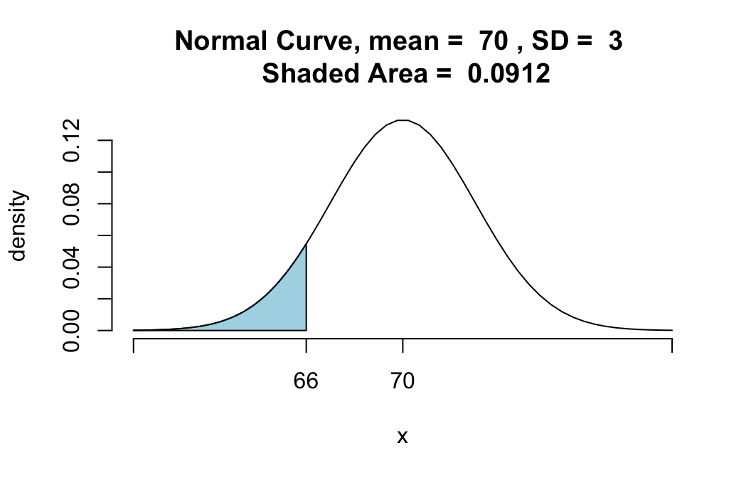

## [1] 0.09121122

You should ask for a graph until you are confident of being able to use pnormGC() to get exactly the probability that you want.

Find P(X > x)

For the same random variable \(X \sim norm(70,3)\), suppose we want the probability that \(X\) is greater than 69, i.e.:

\[P(X > 69).\]

Ask for:

pnormGC(bound=69,region="above",
        mean=70,sd=3,graph=TRUE)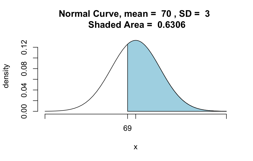

## [1] 0.6305587

Finding P(a < X < b)

For the same random variable \(X \sim norm(70,3)\), suppose we want the probability that \(X\) is between 68 and 72, i.e.:

\[P(68 < X < 72).\]

Ask for:

pnormGC(bound=c(68,72),region="between",
        mean=70,sd=3,graph=TRUE)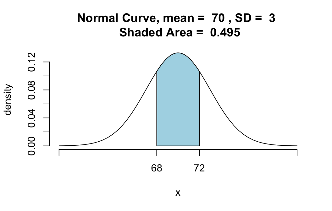

## [1] 0.4950149

Observe that since there are two numbers—68 and 72—that are boundaries, we have to specify both of them for pnormGC() in the form of a list c(68,72).

“Outside” Probabilities

For the same random variable \(X \sim norm(70,3)\), suppose we want the probability that either \(X\) is less than 66 OR that \(X\) is more than 73. Then we are looking for:

\[P(X < 66 \textbf{ or } X > 73).\]

We can find this with the command:

pnormGC(bound=c(66,73),region="outside",
         mean=70,sd=3,graph=TRUE)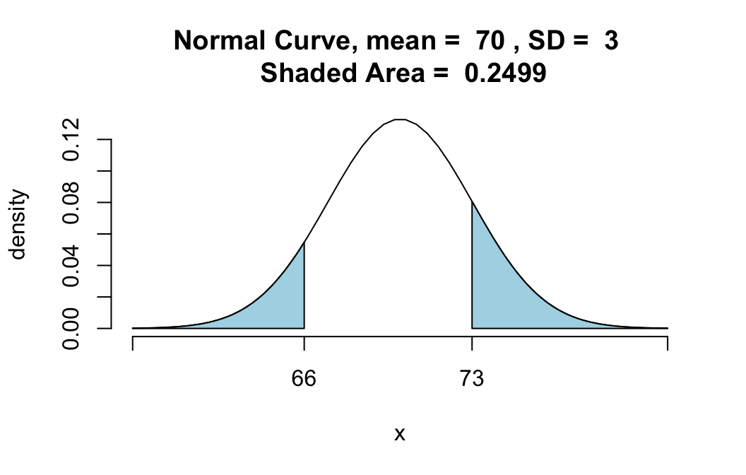

## [1] 0.2498665

Again observe that there are two numbers—66 and 73—that make the boundaries, so supply both of them to the bound argument as a list: c(66,72).

Non-Strict Inequalities

Suppose that for the same random variable \(X \sim norm(70,3)\), you want the probability that \(X\) will turn out to be no more than 66, i.e., you want:

\[P(X \leq 66).\]

You get this with exactly the same function call that gives you \(P(X < 66)\), namely:

pnormGC(bound=66,region="below",
        mean=70,sd=3)

Remember why? Normal random variables are continuous random variables, and for any continuous random variable the chance that it is exactly equal to any particular value is zero. For example, the probability that \(X\) is exactly equal to 66 is given by:

pnormGC(bound=c(66,66),region="between",
        mean=70,sd=3,graph=TRUE)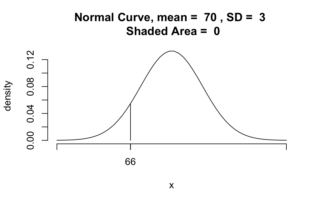

## [1] 0

The probability of getting exactly 66 is given by the area of the line segment under the curve over 66. But the area of a line segment—if you think of it as a “rectangle”" with zero width—is zero!

When you ask for

\[P(X \leq 66)\]

as opposed to

\[P(X < 66),\]

you are adding on just the chance of \(X\) being exactly 66. Since this extra chance is zero, you get the same probability as you did with the strict inequality.