Using ttestGC()
Preliminaries
You use ttestGC() for inferential procedures regarding:
- one population mean \(\mu\);
- the difference of two population means, \(\mu_1 - \mu_2\);
- the mean \(\mu_d\) of paired differences in a population.
The function comes from the tigerstats package, so make sure that tigerstats is loaded:
require(tigerstats)One Mean, From Data Frame (Read This!!)
Read this section carefully. It talks about:
- levels of confidence,
- types of Alternative Hypothesis,
- graphs of the P-value, and
- an option to limit output to the console
in ways that apply to all uses of ttestGC().
Confidence Interval Only
In the m111survey data from the tigerstats package, suppose you want a 95%-confidence interval for:
\(\mu =\) the mean fastest speed ever driven, for all GC students.
Use the function:
ttestGC(~fastest,data=m111survey)##
##
## Inferential Procedures for One Mean mu:
##
##
## Descriptive Results:
##
## variable mean sd n
## fastest 105.9 20.88 71
##
##
## Inferential Results:
##
## Estimate of mu: 105.9
## SE(x.bar): 2.478
##
## 95% Confidence Interval for mu:
##
## lower.bound upper.bound
## 100.959833 110.842984To get any other level of confidence, you need to use the conf.level argument, indicating your desired level of confidence in decimal (not percentage) form.
For example, for a 90%-confidence interval for \(\mu\), use
ttestGC(~fastest,data=m111survey,conf.level=0.90)##
##
## Inferential Procedures for One Mean mu:
##
##
## Descriptive Results:
##
## variable mean sd n
## fastest 105.9 20.88 71
##
##
## Inferential Results:
##
## Estimate of mu: 105.9
## SE(x.bar): 2.478
##
## 90% Confidence Interval for mu:
##
## lower.bound upper.bound
## 101.771329 110.031488Interval and Test
If you want a test of significance as well as the confidence interval, then
- use the
muargument to set what the Null Hypothesis thinks that the value of \(\mu\) is; - use the
alternativeargument to specify the Alternative Hypothesis.
For example, if the hypotheses are:
\(H_0: \mu = 100\)
\(H_a: \mu > 100\)
Then use:
ttestGC(~fastest,data=m111survey,mu=100,alternative="greater")##
##
## Inferential Procedures for One Mean mu:
##
##
## Descriptive Results:
##
## variable mean sd n
## fastest 105.9 20.88 71
##
##
## Inferential Results:
##
## Estimate of mu: 105.9
## SE(x.bar): 2.478
##
## 95% Confidence Interval for mu:
##
## lower.bound upper.bound
## 101.771329 Inf
##
## Test of Significance:
##
## H_0: mu = 100
## H_a: mu > 100
##
## Test Statistic: t = 2.382
## Degrees of Freedom: 70
## P-value: P = 0.009974If the hypotheses are:
\(H_0: \mu = 100\)
\(H_a: \mu < 100\)
Then use:
ttestGC(~fastest,data=m111survey,mu=100,alternative="less")##
##
## Inferential Procedures for One Mean mu:
##
##
## Descriptive Results:
##
## variable mean sd n
## fastest 105.9 20.88 71
##
##
## Inferential Results:
##
## Estimate of mu: 105.9
## SE(x.bar): 2.478
##
## 95% Confidence Interval for mu:
##
## lower.bound upper.bound
## -Inf 110.031488
##
## Test of Significance:
##
## H_0: mu = 100
## H_a: mu < 100
##
## Test Statistic: t = 2.382
## Degrees of Freedom: 70
## P-value: P = 0.99If the hypotheses are:
\(H_0: \mu = 100\)
\(H_a: \mu \neq 100\)
Then use:
ttestGC(~fastest,data=m111survey,mu=100,
        alternative="two.sided")
##
##
## Inferential Procedures for One Mean mu:
##
##
## Descriptive Results:
##
## variable mean sd n
## fastest 105.9 20.88 71
##
##
## Inferential Results:
##
## Estimate of mu: 105.9
## SE(x.bar): 2.478
##
## 95% Confidence Interval for mu:
##
## lower.bound upper.bound
## 100.959833 110.842984
##
## Test of Significance:
##
## H_0: mu = 100
## H_a: mu != 100
##
## Test Statistic: t = 2.382
## Degrees of Freedom: 70
## P-value: P = 0.01995But note that the default value of alternative is “two.sided”, so if you want you could just leave it out and still get a two-sided test:
ttestGC(~fastest,data=m111survey,mu=100)Graph of the P-Value
Anytime you want, you can get a graph of the \(P\)-value for your test, simply by setting the argument graph to TRUE:
ttestGC(~fastest,data=m111survey,mu=100,
        alternative="two.sided",graph=TRUE)
##
##
## Inferential Procedures for One Mean mu:
##
##
## Descriptive Results:
##
## variable mean sd n
## fastest 105.9 20.88 71
##
##
## Inferential Results:
##
## Estimate of mu: 105.9
## SE(x.bar): 2.478
##
## 95% Confidence Interval for mu:
##
## lower.bound upper.bound
## 100.959833 110.842984
##
## Test of Significance:
##
## H_0: mu = 100
## H_a: mu != 100
##
## Test Statistic: t = 2.382
## Degrees of Freedom: 70
## P-value: P = 0.01995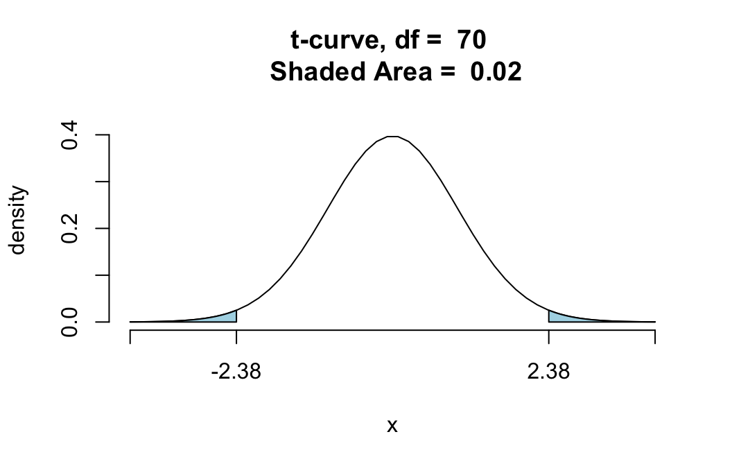
Limiting Output
Sometimes you don’t need R to print so much information to the console. If you want only the basics (such as a confidence interval, the test statistic and \(P\)-value), then set the verbose argument to FALSE:
ttestGC(~fastest,data=m111survey,mu=100,
        alternative="two.sided",verbose=FALSE)
##
##
## Inferential Procedures for One Mean mu:
## 95% Confidence Interval for mu:
##
## lower.bound upper.bound
## 100.959833 110.842984
##
## Test Statistic: t = 2.382
## Degrees of Freedom: 70
## P-value: P = 0.01995One Mean, From Summary Data
Confidence Interval Only
Say that you have taken a simple random sample from some large population, and:
- the sample mean is \(\bar{x}=30\),
- the sample standard deviation is \(s=4\),
- the sample size was \(n=40\).
You don’t have the raw data present in a data frame, but you have enough summary data to use ttestGC(). You just have to set some new arguments:
- set
meanto the sample mean; - set
sdto the sample standard deviation; - set
nto the sample size.
So if you only want a 95%-confidence interval for \(\mu\). use:
ttestGC(mean=30,sd=4,n=40)##
##
## Inferential Procedures for One Mean mu:
##
##
## Descriptive Results:
##
## mean sd n
## 30 4 40
##
##
## Inferential Results:
##
## Estimate of mu: 30
## SE(x.bar): 0.6325
##
## 95% Confidence Interval for mu:
##
## lower.bound upper.bound
## 28.720738 31.279262Interval and Test
If you also want to do a test of significance, again specify mu and alternative. For example, to test the hypotheses
\(H_0: \mu = 32\)
\(H_a: \mu < 32\)
use:
ttestGC(mean=30,sd=4,n=40,
        mu=32,alternative="less")
##
##
## Inferential Procedures for One Mean mu:
##
##
## Descriptive Results:
##
## mean sd n
## 30 4 40
##
##
## Inferential Results:
##
## Estimate of mu: 30
## SE(x.bar): 0.6325
##
## 95% Confidence Interval for mu:
##
## lower.bound upper.bound
## -Inf 31.065609
##
## Test of Significance:
##
## H_0: mu = 32
## H_a: mu < 32
##
## Test Statistic: t = -3.162
## Degrees of Freedom: 39
## P-value: P = 0.001514Difference of Two Means, Data Frame
Confidence Interval Only
Suppose
\(\mu_1 =\) mean fastest speed ever driven, by all GC females
\(\mu_2 =\) mean fastest speed ever driven, by all GC males
If you desire, say, an 85%-confidence interval for \(\mu_1 - \mu_2\), then use:
ttestGC(fastest~sex,data=m111survey,
        conf.level=0.85)
##
##
## Inferential Procedures for the Difference of Two Means mu1-mu2:
## (Welch's Approximation Used for Degrees of Freedom)
## fastest grouped by sex
##
##
## Descriptive Results:
##
## group mean sd n
## female 100.0 17.61 40
## male 113.5 22.57 31
##
##
## Inferential Results:
##
## Estimate of mu1-mu2: -13.4
## SE(x1.bar - x2.bar): 4.918
##
## 85% Confidence Interval for mu1-mu2:
##
## lower.bound upper.bound
## -20.579953 -6.223273Interval and Test
If you want a 95%-confidence interval for \(\mu_1 - \mu_2\) and you would like to test the hypotheses:
\(H_0: \mu_1 - \mu_2 = 0\)
\(H_a: \mu_1 - \mu_2 \neq 0\)
then use:
ttestGC(fastest~sex,data=m111survey,
      mu=0)
##
##
## Inferential Procedures for the Difference of Two Means mu1-mu2:
## (Welch's Approximation Used for Degrees of Freedom)
## fastest grouped by sex
##
##
## Descriptive Results:
##
## group mean sd n
## female 100.0 17.61 40
## male 113.5 22.57 31
##
##
## Inferential Results:
##
## Estimate of mu1-mu2: -13.4
## SE(x1.bar - x2.bar): 4.918
##
## 95% Confidence Interval for mu1-mu2:
##
## lower.bound upper.bound
## -23.254640 -3.548586
##
## Test of Significance:
##
## H_0: mu1-mu2 = 0
## H_a: mu1-mu2 != 0
##
## Test Statistic: t = -2.725
## Degrees of Freedom: 55.49
## P-value: P = 0.008579Notice that this time:
- you specified the Null’s belief about the value of \(\mu_1-\mu_2\) using the
muargument; - you did not have to set
conf.levelto 0.95 (the default value of the argument is 0.95 already); - you did not have to specify the two-sided alternative (the default value of
alternativeis already “two.sided”).
Order of the Groups
Suppose that in the previous situation you had defined:
\(\mu_1 =\) mean fastest speed ever driven, by all GC males
\(\mu_2 =\) mean fastest speed ever driven, by all GC females
Then for you, the first population is all GC males and the second population is all GC females. In order to guarantee that R abides by your choice, use the argument first:
ttestGC(fastest~sex,data=m111survey,
      mu=0,first="male")
##
##
## Inferential Procedures for the Difference of Two Means mu1-mu2:
## (Welch's Approximation Used for Degrees of Freedom)
## fastest grouped by sex
##
##
## Descriptive Results:
##
## group mean sd n
## male 113.5 22.57 31
## female 100.0 17.61 40
##
##
## Inferential Results:
##
## Estimate of mu1-mu2: 13.4
## SE(x1.bar - x2.bar): 4.918
##
## 95% Confidence Interval for mu1-mu2:
##
## lower.bound upper.bound
## 3.548586 23.254640
##
## Test of Significance:
##
## H_0: mu1-mu2 = 0
## H_a: mu1-mu2 != 0
##
## Test Statistic: t = 2.725
## Degrees of Freedom: 55.49
## P-value: P = 0.008579Difference of Two Means, Summary Data
Confidence Interval Only
Suppose that you have taken two independent samples from two populations (or performed a completely randomized experiment with two treatment groups), and you have the following summary data:
| Group | \(\bar{x}\) | \(s\) | \(n\) |
|---|---|---|---|
| group one | 32 | 4.2 | 33 |
| group two | 30 | 5.1 | 42 |
You need to provide the summary data to the arguments mean, sd and n, as lists using the c() function. In each list, data from the first group should come first.
For a 95%-confidence interval for \(\mu_1 - \mu_2\), use:
ttestGC(mean=c(32,30),sd=c(4.2,5.1),n=c(33,42))##
##
## Inferential Procedures for the Difference of Two Means mu1-mu2:
## (Welch's Approximation Used for Degrees of Freedom)
## Results from summary data.
##
##
## Descriptive Results:
##
## group mean sd n
## Group 1 32 4.2 33
## Group 2 30 5.1 42
##
##
## Inferential Results:
##
## Estimate of mu1-mu2: 2
## SE(x1.bar - x2.bar): 1.074
##
## 95% Confidence Interval for mu1-mu2:
##
## lower.bound upper.bound
## -0.140898 4.140898Interval and Test
Suppose that you want a 90%-confidence interval for \(\mu_1 - \mu_2\) and that you would like to test the hypotheses:
\(H_0: \mu_1 - \mu_2 = 0\)
\(H_a: \mu_1 - \mu_2 > 0\)
Suppose also that want a graph of the \(P\)-value. Then use:
ttestGC(mean=c(32,30),sd=c(4.2,5.1),n=c(33,42),
        mu=0,alternative="greater",
        conf.level=0.90,graph=TRUE)
##
##
## Inferential Procedures for the Difference of Two Means mu1-mu2:
## (Welch's Approximation Used for Degrees of Freedom)
## Results from summary data.
##
##
## Descriptive Results:
##
## group mean sd n
## Group 1 32 4.2 33
## Group 2 30 5.1 42
##
##
## Inferential Results:
##
## Estimate of mu1-mu2: 2
## SE(x1.bar - x2.bar): 1.074
##
## 90% Confidence Interval for mu1-mu2:
##
## lower.bound upper.bound
## 0.610797 Inf
##
## Test of Significance:
##
## H_0: mu1-mu2 = 0
## H_a: mu1-mu2 > 0
##
## Test Statistic: t = 1.862
## Degrees of Freedom: 72.82
## P-value: P = 0.03333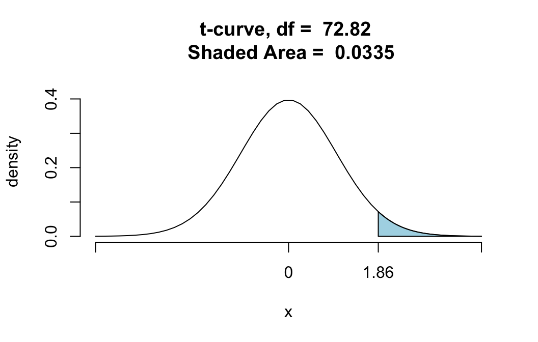
Mean of Differences
Both Variables in the Data Frame
Confidence Interval Only
Suppose that
\(\mu_d =\) mean difference (ideal height minus actual height) for all Georgetown College student.
Both of the relevant variables—ideal_ht and height—are present in the m111survey data frame.
If you want a 95%-confidence interval for \(\mu_d\), then use:
ttestGC(~ideal_ht - height,data=m111survey)##
##
## Inferential Procedures for the Difference of Means mu-d:
## ideal_ht minus height
##
##
## Descriptive Results:
##
## Difference mean.difference sd.difference n
## ideal_ht - height 1.946 3.206 69
##
##
## Inferential Results:
##
## Estimate of mu-d: 1.946
## SE(d.bar): 0.3859
##
## 95% Confidence Interval for mu-d:
##
## lower.bound upper.bound
## 1.175528 2.715776Note how the “~” character signals the presence of a formula.
Interval and Test
In order to test:
\(H_0: \mu_d = 0\)
\(H_a: \mu_d > 0\)
use:
ttestGC(~ideal_ht - height,data=m111survey,
        mu=0,alternative="greater")
##
##
## Inferential Procedures for the Difference of Means mu-d:
## ideal_ht minus height
##
##
## Descriptive Results:
##
## Difference mean.difference sd.difference n
## ideal_ht - height 1.946 3.206 69
##
##
## Inferential Results:
##
## Estimate of mu-d: 1.946
## SE(d.bar): 0.3859
##
## 95% Confidence Interval for mu-d:
##
## lower.bound upper.bound
## 1.302075 Inf
##
## Test of Significance:
##
## H_0: mu-d = 0
## H_a: mu-d > 0
##
## Test Statistic: t = 5.041
## Degrees of Freedom: 68
## P-value: P = 1.826e-06The Difference is in the Data Frame
Sometimes the difference of the two relevant numerical variables is included in the data frame as another variable: such is the case for m111survey, where the difference is recorded as the variable diff.ideal.act.
If you would like to use this difference, then work just as if you were studying one population mean \(\mu\).
Confidence Interval Only
Thus, for a 95%-confidence interval for \(\mu_d\) we could also have done:
ttestGC(~diff.ideal.act.,data=m111survey)##
##
## Inferential Procedures for One Mean mu:
##
##
## Descriptive Results:
##
## variable mean sd n
## diff.ideal.act. 1.946 3.206 69
##
##
## Inferential Results:
##
## Estimate of mu: 1.946
## SE(x.bar): 0.3859
##
## 95% Confidence Interval for mu:
##
## lower.bound upper.bound
## 1.175528 2.715776Interval and Test
For a test of
\(H_0: \mu_d = 0\)
\(H_a: \mu_d > 0\)
we could have done:
ttestGC(~diff.ideal.act.,data=m111survey,
        mu=0,alternative="greater")
##
##
## Inferential Procedures for One Mean mu:
##
##
## Descriptive Results:
##
## variable mean sd n
## diff.ideal.act. 1.946 3.206 69
##
##
## Inferential Results:
##
## Estimate of mu: 1.946
## SE(x.bar): 0.3859
##
## 95% Confidence Interval for mu:
##
## lower.bound upper.bound
## 1.302075 Inf
##
## Test of Significance:
##
## H_0: mu = 0
## H_a: mu > 0
##
## Test Statistic: t = 5.041
## Degrees of Freedom: 68
## P-value: P = 1.826e-06Note that in its statement of hypotheses, R identifies the parameter of interest as \(\mu\) rather than as \(\mu_d\). It had no way of knowing that diff.ideal.act. recorded the difference of a pair of measurements.