Using binomtestGC()
Preliminaries
You use binomtestGC() for inferential procedures regarding one population proportion \(p\). The function proptestGC() can also handle this analysis, but binomtestGC() computes exact \(P\)-values rather than employing the (sometimes crude) normal approximation, and it also uses a somewhat more sophisticated method to compute confidence intervals.
Make sure you have tigerstats loaded:
require(tigerstats)Working from a Data Frame
Let
\(p =\) the proportion of all Georgetown College students who are female
Suppose that you would like a 95%-confidence interval for \(p\). Since sex is present as a variable in the m111survey data frame, you can use formula-data input in the usual way to direct the attention of binomtestGC() to sex as the data.
However, when the function looks at sex, it sees the values “female” and “male”. It needs to be told which of them to count as a “success” when it computes the sample proportion \(\hat{p}\). You do this with the success argument.
So you use:
binomtestGC(~sex,data=m111survey,
            success="female")
## Exact Binomial Procedures for a Single Proportion p:
## Variable under study is sex
##
## Descriptive Results: 40 successes in 71 trials
##
## Inferential Results:
##
## Estimate of p: 0.5634
## SE(p.hat): 0.0589
##
## 95% Confidence Interval for p:
##
## lower.bound upper.bound
## 0.440455 0.680850Note that you did not have to specify a confidence level: by default, the function returns a 95%-confidence interval.
Setting the Confidence Level
You can get intervals with other levels of confidence besides 95%, simply by setting the argument conf.level to the desired level (expressed as a proportion, rather than as a percentage).
For example, if you want a 90%-confidence interval for \(p\), then you use:
binomtestGC(~sex,data=m111survey,
            success="female",conf.level=0.90)
## Exact Binomial Procedures for a Single Proportion p:
## Variable under study is sex
##
## Descriptive Results: 40 successes in 71 trials
##
## Inferential Results:
##
## Estimate of p: 0.5634
## SE(p.hat): 0.0589
##
## 90% Confidence Interval for p:
##
## lower.bound upper.bound
## 0.458929 0.663741Significance Tests
Let’s now let
\(p =\) the proportion of all Georgetown College students who are male
(Notice that, for variety’s sake, we have switched to counting up males.)
Suppose that we want to perform a test of significance. Then we would use:
- the argument
pto indicate the belief of the Null Hypothesis as to the value of \(p\); - the argument
alternativeto specify the direction of the Alternative Hypothesis. The possible values of this argument are:- “less”
- “greater”
- “two.sided” (the default value)
For example, if we want to test the hypotheses:
\(H_0 : p = 0.50\)
\(H_a : p < 0.50\)
then we use
binomtestGC(~sex,data=m111survey,
            success="male",p=0.50,
            alternative="less")
## Exact Binomial Procedures for a Single Proportion p:
## Variable under study is sex
##
## Descriptive Results: 31 successes in 71 trials
##
## Inferential Results:
##
## Estimate of p: 0.4366
## SE(p.hat): 0.0589
##
## 95% Confidence Interval for p:
##
## lower.bound upper.bound
## 0.000000 0.541071
##
## Test of Significance:
##
## H_0: p = 0.5
## H_a: p < 0.5
##
## P-value: P = 0.1712To test the hypotheses
\(H_0 : p = 0.50\)
\(H_a : p > 0.50\)
then we use
binomtestGC(~sex,data=m111survey,
            success="male",p=0.50,
            alternative="greater")
## Exact Binomial Procedures for a Single Proportion p:
## Variable under study is sex
##
## Descriptive Results: 31 successes in 71 trials
##
## Inferential Results:
##
## Estimate of p: 0.4366
## SE(p.hat): 0.0589
##
## 95% Confidence Interval for p:
##
## lower.bound upper.bound
## 0.336259 1.000000
##
## Test of Significance:
##
## H_0: p = 0.5
## H_a: p > 0.5
##
## P-value: P = 0.8825If we want a two-side test
\(H_0 : p = 0.50\)
\(H_a : p \neq 0.50\)
then we use
binomtestGC(~sex,data=m111survey,
            success="male",p=0.50)
## Exact Binomial Procedures for a Single Proportion p:
## Variable under study is sex
##
## Descriptive Results: 31 successes in 71 trials
##
## Inferential Results:
##
## Estimate of p: 0.4366
## SE(p.hat): 0.0589
##
## 95% Confidence Interval for p:
##
## lower.bound upper.bound
## 0.319150 0.559545
##
## Test of Significance:
##
## H_0: p = 0.5
## H_a: p != 0.5
##
## P-value: P = 0.3425Note that there is no need to specify an alternative, since the default value of alternative is “two.sided”.
A Graph of the \(P\)-Value
We can get a graph of the \(P\)-value simply by setting the argument graph to TRUE:
binomtestGC(~sex,data=m111survey,
            success="male",p=0.50,
            alternative="less",
            graph=TRUE)
## Exact Binomial Procedures for a Single Proportion p:
## Variable under study is sex
##
## Descriptive Results: 31 successes in 71 trials
##
## Inferential Results:
##
## Estimate of p: 0.4366
## SE(p.hat): 0.0589
##
## 95% Confidence Interval for p:
##
## lower.bound upper.bound
## 0.000000 0.541071
##
## Test of Significance:
##
## H_0: p = 0.5
## H_a: p < 0.5
##
## P-value: P = 0.1712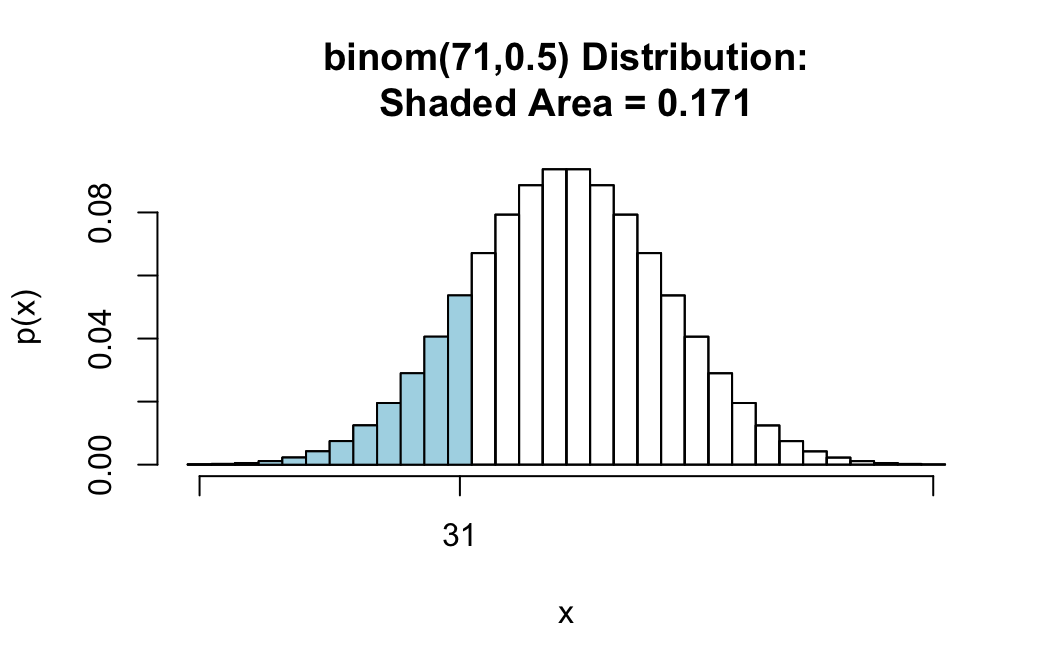
Working with Summary Data
Suppose that in a poll of 2500 randomly selected registered voters, 1325 of them indicated support for the Affordable Care Act. Suppose that we want a confidence interval for \(p\), the proportion of all registered voters who favor the Act, and a two-sided test of significance with the hypotheses:
\(H_0 : p = 0.50\)
\(H_a : p \neq 0.50\)
We do not have raw data from a data frame, but the summary information we are given will suffice for binomtestGC(). We need only:
- set the argument
xto the number of successes (the count of people who said they support the Act), and - set the argument
nto the sample size.
Hence we use:
binomtestGC(x=1325,n=2500,p=0.50)## Exact Binomial Procedures for a Single Proportion p:
## Results based on Summary Data
##
## Descriptive Results: 1325 successes in 2500 trials
##
## Inferential Results:
##
## Estimate of p: 0.53
## SE(p.hat): 0.01
##
## 95% Confidence Interval for p:
##
## lower.bound upper.bound
## 0.510210 0.549719
##
## Test of Significance:
##
## H_0: p = 0.5
## H_a: p != 0.5
##
## P-value: P = 0.0029Want Less Output?
Sometimes you don’t need to see quite so much output to the console. If you only want the basics (confidence interval for \(p\) and \(P\)-value for your test), then set the argument verbose to FALSE.
For example, if you want a 90%-confidence interval and a two-sided test then try:
binomtestGC(~sex,data=m111survey,
            success="male",p=0.50,
            verbose=FALSE)
## Exact Binomial Procedures for a Single Proportion p:
## Variable under study is sex
## 95% Confidence Interval for p:
##
## lower.bound upper.bound
## 0.319150 0.559545
##
## P-value: P = 0.3425