Chapter 7 Basic Probability

7.1 Introduction

Statistical inference is the process of forming judgments about a population based on information gathered from a sample of that population. Our goal in this chapter is to describe populations and samples using the language of probability.

7.2 Probability

By probability, we mean some number between 0 and 1 that describes the likelihood, or chance, that an event occurs. Probability is a way to quantify uncertainty.

There are several different interpretations of the word probability that come from understanding how the numbers are generated.

7.2.1 Subjective Probability

Subjective Probabilbities: Probabilities that are assigned or postulated based on a personal belief that an outcome will occur are called subjective probabilities.

Example: A surgeon, who is performing a surgery for the very first time, tells his patient that he feels that the probability that it will be successful is 0.99. This probability is subjective because it is based entirely on the surgeon’s belief.

In this class, we will not be very interested in subjective probabilities since they are not supported by data.

7.2.2 Theoretical Probability

To discuss theoretical probabilities, let’s first state some definitions.

Sample Space: The sample space is the set of all possible outcomes of ane experiment.
Event: An event is a subset of the sample space. In other words, an event is a collection of outcomes.

Suppose that all outcomes in a sample space are equally likely - i.e. they have the same chance of occurring. Then, the probability of an event is the number of outcomes in the event divided by the total number of outcomes in the sample space. In symbols, this is

\[\mbox{P(event)} = \dfrac{\mbox{number of outcomes in the event}}{\mbox{total number of outcomes in the sample space}}.\]

Example: Consider tossing a fair coin. There are two possible outcomes - tossing a head or tossing a tail. The sample space is the set of all possible outcomes, so the sample space is {H, T}. Since the coin is fair, the outcomes are equally likely. The probability of the event toss a head is $\dfrac{1}{2}=0.5$. In symbols, we can write this as $\mbox{P(toss a head)}=0.5$ or, for short, $\mbox{P(H)}=0.5$.

Example: Consider tossing two fair coins. The sample space is {HH, HT, TH, TT}. Here, HH represents both coins landing heads up and TH represents the first coin landing tails and second coin landing H. Since the coin is fair, each of the four outcomes is equally likely. We can compute various probabilities.

What is $\mbox{P(HH)}$?

Answer: $\mbox{P(HH)}=\dfrac{1}{4}=0.25$. This is the probability of tossing 2 heads in two tosses of a fair coin. One of the four events in the sample space corresponds to 2 heads being tossed - HH.

What is the probability of tossing exactly one head?

Answer: $\mbox{P(toss exactly one head)}=\mbox{P(HT or TH)} = \dfrac{2}{4}=0.5$. This is the probability of tossing exactly 1 heads in two tosses of a fair coin. Two of the four events in the sample space corresponds to exactly 1 head being tossed - HT, TH.

What is the probability of getting a head on the first toss?

Answer: $\mbox{P(toss a head on Toss 1)}=\mbox{P(HT or HH)} = \dfrac{2}{4}=0.5$. This is the probability of tossing a head on the first toss in two tosses of a fair coin. Two of the four events in the sample space corresponds to this - HT, HH.

7.2.3 Long-run Frequency Probability

The final type of probability we should discuss is really an approximation to the theoretical probability.

Long-Run Frequency Probability: A long-run frequency probability comes from knowing the proportion of times that the event occurs when the experiment is performed over and over again. This is an approximation to a theoretical probability.

Example: Suppose you toss a fair coin 1000 times and it comes up as a tail 502 times. Then the long run frequency is $\dfrac{502}{1000}=0.502$. We know that the theoretial (true) probability of a fair coin landing heads is 0.50. The long run frequency is an approximation this. The more times the coin is tossed, the better the long run frequency does at approximating the true probability of landing tails.

7.3 What is a Random Variable?

Here is a very important definition:

Random Variable: A random variable is a variable whose value is the outcome of a chance experiment.

Calling it a variable may be somewhat confusing! It is actually a function on the sample space of an experiment. It can take on a set of possible different values. We make a distinction between whether or not we know, or have observed, the value of the random variable. Once observed, the random variable is known. Prior to being observed, it is full of potential - it can take on any value in the set of possible values. However, some of the possible values may be more likely than others. There is an associated probability that the random variable is equal to some value (or is in some range of values).

7.3.1 Notation

Letters near the end of the alphabet are typically used to symbolize a random variable. If the random variable has not yet been observed, we use uppercase letters, such as $X$, $Y$, and $Z$. If the value of the random variable is known, we use lowercase letters, such as $x$, $y$, and $z$, to refer to the random variable.

Just as numeric data is either discrete or continuous, random variables are classified as either discrete or continuous. This is determined by what kinds of numbers are in the set of possible values that the random variable can assume.

7.4 Discrete Random Variables

Discrete random Variable: A discrete random variable is a random variable whose possible values come from a set of discrete numbers.

Example: Suppose that we toss a fair coin two times.

The sample space is {HH, HT, TH, TT}.
A possible random variable associated with this experiment is $X=\mbox{ number of heads tossed}$.
The set of possible values that $X$ can assume is {0, 1, 2}. Since this is a set of discrete values, we classify $X$ as a discrete random variable.
Recall that there is an associated probability that the random variable is equal to some value. For this example, it is more likely that $X=1$ than $X=0$ or $X=2$. This can be seen by looking at the probabilities:
- $\mbox{P}(X=0)=1/4=0.25$. Keep in mind that $X$ is the random variable that represents the “number of heads tossed in two tosses of a fair coin”. This is just another way to represent the $\mbox{P(TT)}$.
- $\mbox{P}(X=1)=2/4=0.5$. This is just another way to represent .
- $\mbox{P}(X=2)=1/4=0.25$. This is just another way to represent the $\mbox{P(HH)}$.

7.4.1 Probability Distribution Functions for Discrete Random Variables

It is nice to display the probabilities associated with a random variable in a table or graph.

Probability Distribution Function (pdf): The probability distribution function (pdf, for short) for a discrete random variable $X$ is a function that assigns probabilities to the possible values of $X$. It may be viewed in the form of a table or a histogram.

For the two-coin toss example, the pdf for the random variable $X=\mbox{ number of heads tossed}$ looks like:

Probability distribution function for two-coin toss
$x$	0	1	2
$P(X=x)$	0.25	0.50	0.25

From the pdf, we can easily see that the probabilities of all possible values of a discrete random variable add up to 1.

\[ \sum \mbox{P}(X=x)=1 \]

We can use a histogram (See Figure[Two Coin Toss pdf]) to visualize the pdf where

the possible outcomes for the random variable $X$ are placed on the horizontal axis,
the probabilities for the possible outcomes are placed on the vertical axis, and
a bar is centered on each possible value and its height is equal to the probability of that value.

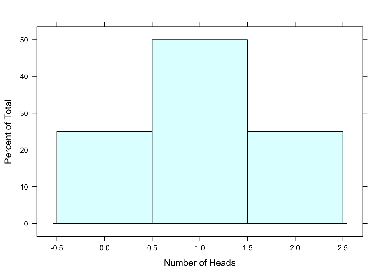
Figure 7.1: Two Coin Toss pdf: The probability distribution function, in histogram form, for a two coin toss.

We can use the pdf and the histogram of the two coin toss example to calculate probabilities.

Example: $\mbox{P}(X = 1)=0.5$. This is the probability of tossing exactly 1 head in two tosses of a fair coin. This corresponds to the area of the pink rectangle in the histogram shown below. See Figure[Exactly 1 Head].

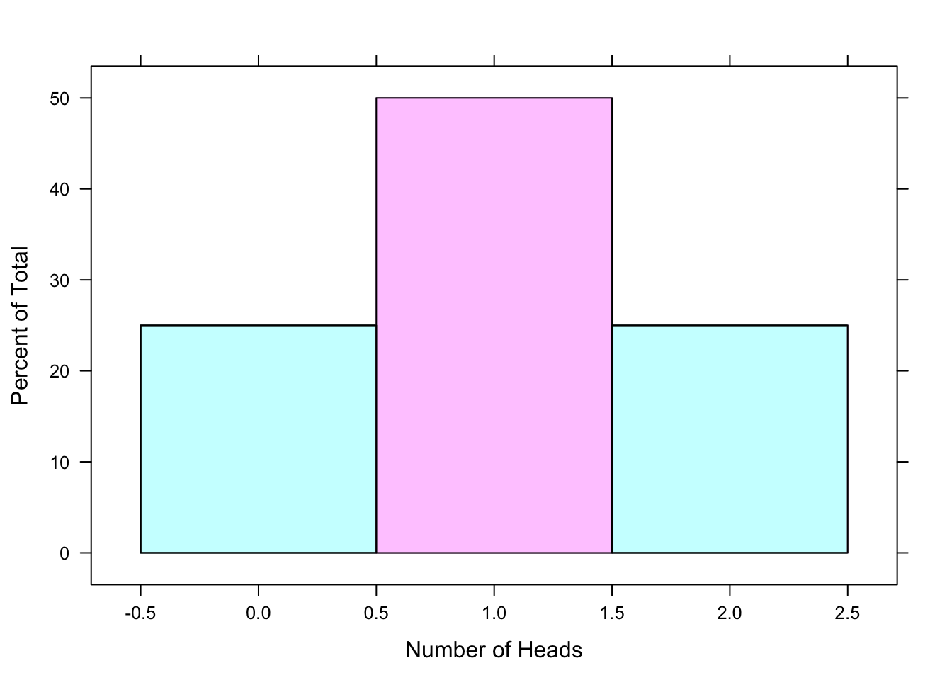
Figure 7.2: Exactly 1 Head: The shaded region of the pdf represents the probability of tossing exactly 1 head in two tosses of a fair coin.

Example: $\mbox{P}(X\geq 1)=0.5+0.25=0.75$. This is the probability of tossing at least 1 head in two tosses of a fair coin. At least 1 head means that you toss 1 head OR 2 heads. In two tosses of a fair coin, the chance that you will toss 1 head is 0.5 and the chance that you will toss 2 heads is 0.25. So the likelihood that you will toss 1 OR 2 heads is 0.5 + 0.25 = 0.75. This corresponds to summing the area of the pink rectangles in the histogram shown below. See Figure[At Least 1 Head].

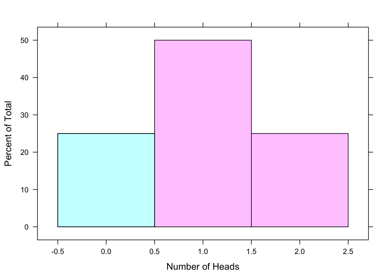
Figure 7.3: At Least 1 Head: The shaded region of the pdf represents the probability of tossing at least 1 head in two tosses of a fair coin.

Example: $\mbox{P}(X \leq 1)=0.25 +0.5=0.75$. This is the probability of tossing at most 1 head in two tosses of a fair coin. At most one head means that we toss 0 heads OR 1 head. In two tosses of a fair coin, the chance that you will toss 0 heads is 0.25 and the chance that you will toss 1 head is 0.5. So the likelihood that you will toss 0 OR 1 head is 0.25 + 0.5 = 0.75. This is called a cumulative probability - it’s the probability that a random variable is less than or equal to some value. This corresponds to summing the area of the pink rectangles in the histogram shown below. See Figure[At Most 1 Head].

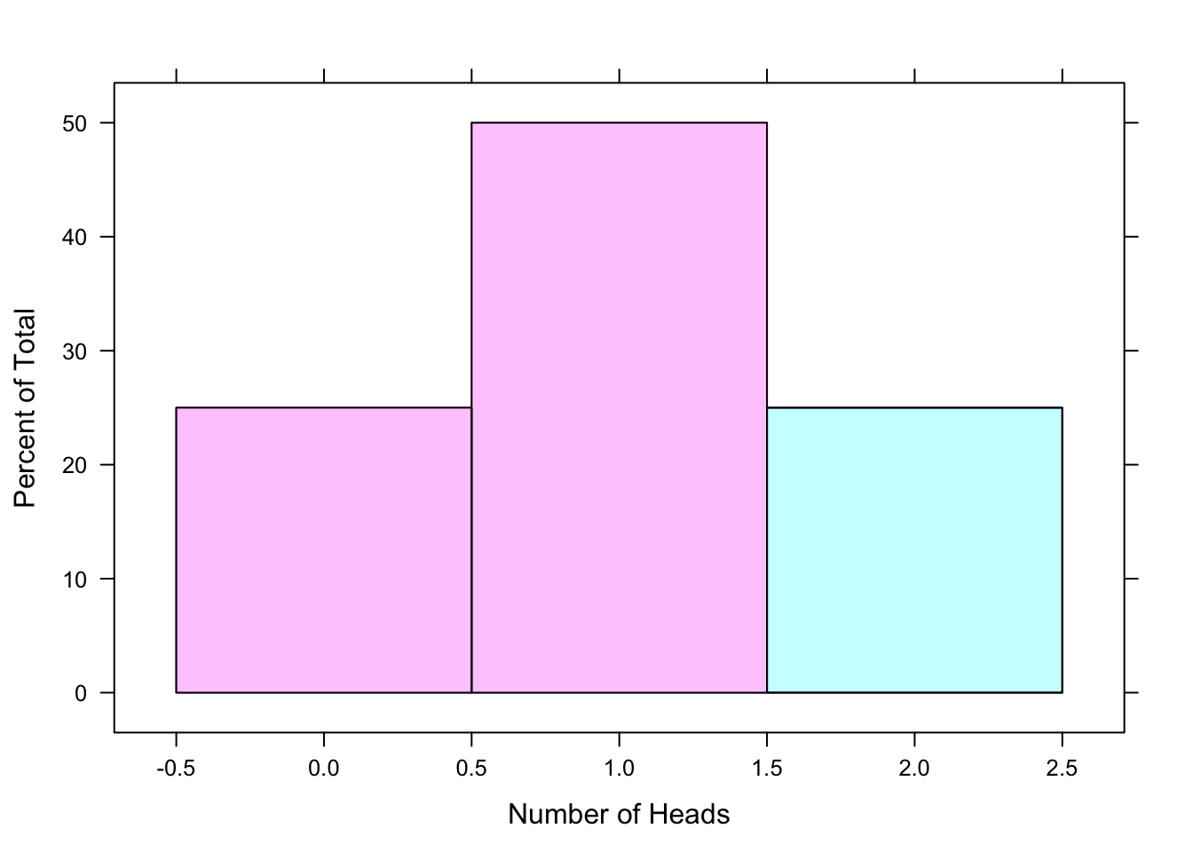
Figure 7.4: At Most 1 Head: The shaded region of the pdf represents the probability of tossing at most 1 head in two tosses of a fair coin.

7.4.2 Expectation of Discrete Random Variables

So far, we have talked about the possible values that a random variable might be. We have also talked about the probability, or chance, that the random variable equals one of those values. Some of the possible values for a random variable are more likely than others. This prompts the question: In the long run, what value do we expect the random variable to be?

Let’s return to our two coin toss and recap what we know.

If our random variable $X=\mbox{number of heads tossed in two tosses of a fair coin}$, then the possible values for $X$ are {0, 1, 2}.
We’ve also found that $X$ is more likely to be 1 than it is to be 0 or 2.
So, if we repeated the two coin toss over and over again, we would expect to see $X=1$ more often than $X=0$ or $X=2$.

Expected Value: The expected value of a random variable $X$ is the value of $X$ that we would expect to see if we repeated our experiment many times.

Expected value is like an average, of sorts. In fact, it’s a weighted average. Each possible value of $X$ is weighted by the likelihood that $X$ is that value. The expected value of $X$, $\mbox{E}(X)$, can be calculated by the formula.

\[\mbox{E}(X)=\sum x\cdot \mbox{P}(X=x)\]

Step by step, this is:

Multiply every possible value for $X$ by it’s corresponding probability.
Sum these products.

For our two coin toss example, the expected value of $X$ can be found with the following R code.

x<-c(0,1,2) #Possible values for X.
prob.x<-c(0.25,0.5,0.25) #Corresponding probabilities 
EV.X<-sum(x*prob.x) #Expected Value of X.
EV.X

## [1] 1

It turns out that $\mbox{E}(X)=$ 1, exactly as we had thought!

7.4.3 Standard Deviation of Discrete Random Variables

Another measure that we are interested in is the standard deviation for random variables.

Standard Deviation: The standard deviation is a measurement of how much the random variable random variable can be expected to differ from its expected value.

In other words, if we repeat an experiment over and over, the standard deviation of a random variable is the average distance that it will fall from its expected value. Of course, this average is weighted by the probabilities. The standard deviation of $X$, $\mbox{SD}(X)$, can be calculated by the formula.

\[\mbox{SD}(X)=\sqrt{\sum \bigg(x-\mbox{E}(X)\bigg)^2\cdot \mbox{P}(X=x)}\]

Step by step, this is:

Calculate the difference between each of the possible values for $X$ and the expected value for $X$.
Square these differences.
Multiply the squared differences by the probability that $X$ equals that value.
Sum these products.
Take the square root.

For our two coin toss example, the standard deviation of $X$ can be found with the following R code.

x<-c(0,1,2) #Possible values for X.
prob.x<-c(0.25,0.5,0.25) #Corresponding probabilities.
EV.X<-sum(x*prob.x) #Expected value of X.  
SD.X<-sqrt(sum((x-EV.X)^2*prob.x)) #Standard deviation of X.  
SD.X

## [1] 0.7071068

So, if we toss a fair coin two times, the number of heads that we would expect to toss is 1. On average, the number of heads will differ from 1 by 0.7071068.

7.4.4 Using EV and SD to Evaluate a Game

The expected value and standard deviation work together to describe how a random variable is likely to turn out. This comes in handy for situations like the following example.

Example: Suppose that you decide to invest $100 in a scheme that will hopefully make you some money. You have 2 investment options, Plan 1 and Plan 2. Let the random variable $X=\mbox{net gain from Plan 1}$ and the random variable $Y=\mbox{net gain from Plan 2}$. The probability distribution functions for the plans are shown below.

Plan 1:

Probability Distribution Function for Investment Plan 1
x	$5,000	$1,000	$0
$P(X=x)$	0.001	0.005	0.994

Plan 2:

Probability Distribution Function for Investment Plan 2
y	$20	$10	$4
$P(Y=y)$	0.30	0.20	0.50

Which plan do you choose? Plan 1 is the riskier plan. You have a chance to get rich off of your investment, but it’s also very likely that will gain nothing! On the other hand, Plan 2 is a safe plan. You won’t get rich, but you are guaranteed to gain some money.

Putting personal desires aside, let’s think about this mathematically by calculating the expected value of each plan.

*Coding Tip:* Since we want to calculate the expected value for 2 different random variables, it’s a good idea to name these variables something slightly different. This helps to keep track of which random variable we’re talking about.

#EV Plan 1
x1 = c(5000, 1000, 0)
prob.x1 = c(0.001, 0.005, 0.994)
EV.X1 = sum(x1 * prob.x1)
EV.X1

## [1] 10

#EV Plan 2
x2 = c(20, 10, 4)
prob.x2 = c(0.30, 0.20, 0.50)
EV.X2 = sum(x2 * prob.x2)
EV.X2

## [1] 10

The expected amount of money you gain from investing in Plan 1 is $10. So, if you could invest your $100 in Plan 1 over and over again, on average you would walk away with a net gain of $10.

The expected gain from investing in Plan 2 is also $10. So, if you could invest your $100 in Plan 2 over and over again, on average you would also have a net gain of $10.

Based on expected values, it seems that the plans are the same! Before you get too excited and invest all of your money in the plan with the highest possible reward, let’s compare the standard deviations. This will give us an idea about how much the net gain for each plan will differ, on average, from the expected value.

#SD Plan 1
x1 = c(5000, 1000, 0)
prob.x1 = c(0.001, 0.005, 0.994)
EV.X1 = sum(x1 * prob.x1)
SD.X1=sqrt(sum((x1-EV.X1)^2*prob.x1))
SD.X1

## [1] 172.9162

#SD Plan 2
x2 = c(20, 10, 4)
prob.x2 = c(0.30, 0.20, 0.50)
EV.X2 = sum(x2 * prob.x2)
SD.X2=sqrt(sum((x2-EV.X2)^2*prob.x2))
SD.X2

## [1] 6.928203

Now, we have a better idea of how $X$ and $Y$ are likely to turn out!

The net gain for Plan 1, $X$, has an expected value of $10 with a standard deviation of $172.92.
The net gain for Plan 2, $Y$, has an expected value of $10 with a standard deviation of $6.93.

Knowing all of this, which plan would you choose?

7.4.5 Independence

Independence: Two events are considered independent if the outcome of one event does not affect the outcome of the other.

Suppose that we draw two cards from a standard 52-card deck. We want to know the probability of drawing a Jack.

If we draw the cards with replacement, then we draw a card from the deck, record the result, and replace the card before we draw again. In other words, we return the deck to it’s original state before drawing the second card. This ensures that the probability of drawing a Jack on the first try is the same as the probability of drawing a Jack on the second try.

$\mbox{P(first draw is a Jack)}=\frac{4}{52}$ and $\mbox{P(second draw is a Jack)}=\frac{4}{52}$. The outcome of our first try did not affect the outcome of our second try. Drawing with replacement makes our two draws independent.

On the other hand, if we draw the cards without replacement, then we do not return the first card to the deck before drawing the second card. The first draw is as before, so $\mbox{P(first draw is a Jack)}=\frac{4}{52}$. However, now the state of the deck has been changed, so the chance of drawing a Jack on the second try depends on what happened on the first try.

If our first draw was a Jack, then the deck is left with only 3 Jacks out of 51 total cards. So, $\mbox{P(second draw is a Jack given that the first draw was a Jack)}=\frac{3}{51}$.

If our first draw was not a Jack, then the deck is left with 4 Jacks out of 51 total cards. So, $\mbox{P(second draw is a Jack given that the first draw was not a Jack)}=\frac{4}{51}$. Drawing without replacement makes our two draws dependent.

7.4.6 A Special Discrete Random Variable: Binomial Random Variable

The coin toss example that we have been looking at is actually an example of a special type of discrete random variable called a binomial random variable.

Binomial Random Variable: A binomial random variable is a random variable that counts how often a particular event occurs in a specified number of tries.

To be a binomial random variable, a random variable must meet all of the following conditions:

There are a specified number of tries. This is sometimes referred to as “size”.
On each try, the event of interest either occurs or it does not. In other words, we have a success or a failure on each try.
The probability of success is the same on each try. (We will denote the probability of success as $p$. In each trial, you will either succeed or you will fail, so the probability of failure will be the complement of a success: $1-p$.)
The tries are independent of one another.

Let’s revisit the two coin toss example using the language of a binomial random variable. Suppose we toss a fair coin twice and let the random variable $X=\mbox{number of heads tossed}$. This is a binomial random variable because it fits the 4 conditions:

Since we are tossing the coin twice, the specified number of trials, or size, is $n=2$.
Each toss is either heads (success) or tails (failure). Since it is a fair coin, the probability of success is $p=0.5$ and the probability of failure is $1-p=1-0.5=0.5$.
The chance of tossing a head is the same on each toss of the coin.
The trials are independent. What you tossed on the first toss does not affect what happens on the second toss.

Let’s try another example.

Example: Suppose we toss a fair coin 5 times. Let the random variable $X=\mbox{number of tails tossed}$. This is a binomial random variable:

Since we are tossing the coin five time, the specified number of trials, or size, is $n=5$.
Each toss is either heads (success) or tails (failure). Since it is a fair coin, the probability of success is $p=0.5$ and the probability of failure is $1-p=1-0.5=0.5$.
The chance of tossing a head is the same on each toss of the coin.
The trials are independent.

Listing out the sample space, and calculating probabilities from it, for a five-coin toss would be rather tedious. There is a function in tigerstats that calculates these probabilities (and produces graphs of the pdf) for us. Let’s calculate a few probabilities using this function pbinomGC.

7.4.6.1 $\mbox{P}(X> 2)$

We will start by calculating $\mbox{P}(X> 2)$. To use pbinomGC we need to supply several inputs:

The bound - for our example, the bound is 2
The region - this is given by the sign in the probability. For our example, we are dealing with >, so our region is "above". Other options for the region are "above", "below", and "outside".
The size - for our example, the number of trials is $n=5$.
The probability of success - for our example, $p=0.5$.
Whether or not you want to display a graph of the probability. The default of this function is to not produce a graph. If you would like to see one, you should include graph=TRUE.

Let’s compute $\mbox{P}(X> 2)$ and view a graph of the probability. See Figure[Binomial Greater Than].

pbinomGC(2,region="above",size=5,prob=0.5,graph=TRUE)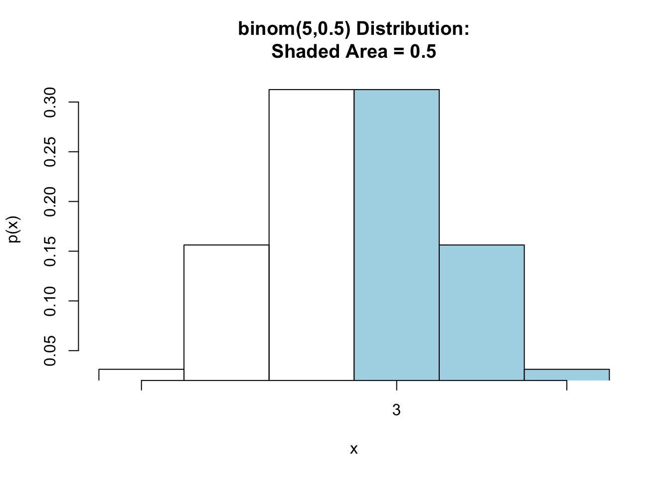

Figure 7.5: Binomial Greater Than: Shaded region represents the probability that more than 2 heads are tossed in 5 tosses of a fair coin.

## [1] 0.5

To just find the probability without producing the graph:

pbinomGC(2,region="above",size=5,prob=0.5)

## [1] 0.5

So, in five tosses of a fair coin, the probability of tossing more than 2 heads is $\mbox{P}(X>2)=$ 0.5.

7.4.6.2 P(X >= 2)

Now, suppose you want to know $P(X\geq 2)$. Since the possible values for $X$ are {0,1,2, 3, 4, 5}, $X\geq 2$ is the same as $X> 1$. The following code will calculate $P(X>1)$. Look at the graph in Figure[Binomial Greater Than or Equal].

pbinomGC(1, region="above",size=5,prob=0.5, graph=TRUE)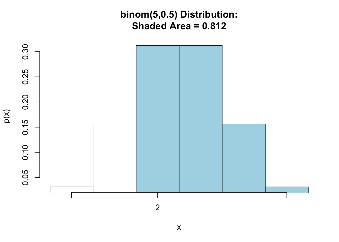

Figure 7.6: Binomial Greater Than or Equal: Shaded region represents the probability that at least 2 heads are tossed in 5 tosses of a fair coin.

## [1] 0.8125

Thus, the probability of tossing at least 2 heads is $\mbox{P}(X\geq 2)=$ 0.8125

7.4.6.3 P(X <= 3)

Now, let’s look at finding the probability that there are at most than 3 heads in five tosses of a fair coin. See Figure[Binomial Less Than or Equal].

pbinomGC(3,region="below",size=5,prob=0.5,graph=TRUE)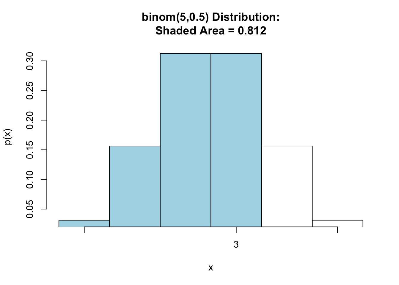

Figure 7.7: Binomial Less Than or Equal: Shaded region represents the probability that at most 3 heads are tossed in 5 tosses of a fair coin.

## [1] 0.8125

Thus, $\mbox{P}(X\leq 3)=$ 0.8125.

7.4.6.4 P(X < 3)

Now, let’s look at finding the probability that there are less than 3 heads in five tosses of a fair coin. Note that for a binomial random variable, $X<3$ is the same as $X\leq 2$. See Figure[Binomial Less Than or Equal].

pbinomGC(2,region="below",size=5,prob=0.5,graph=TRUE)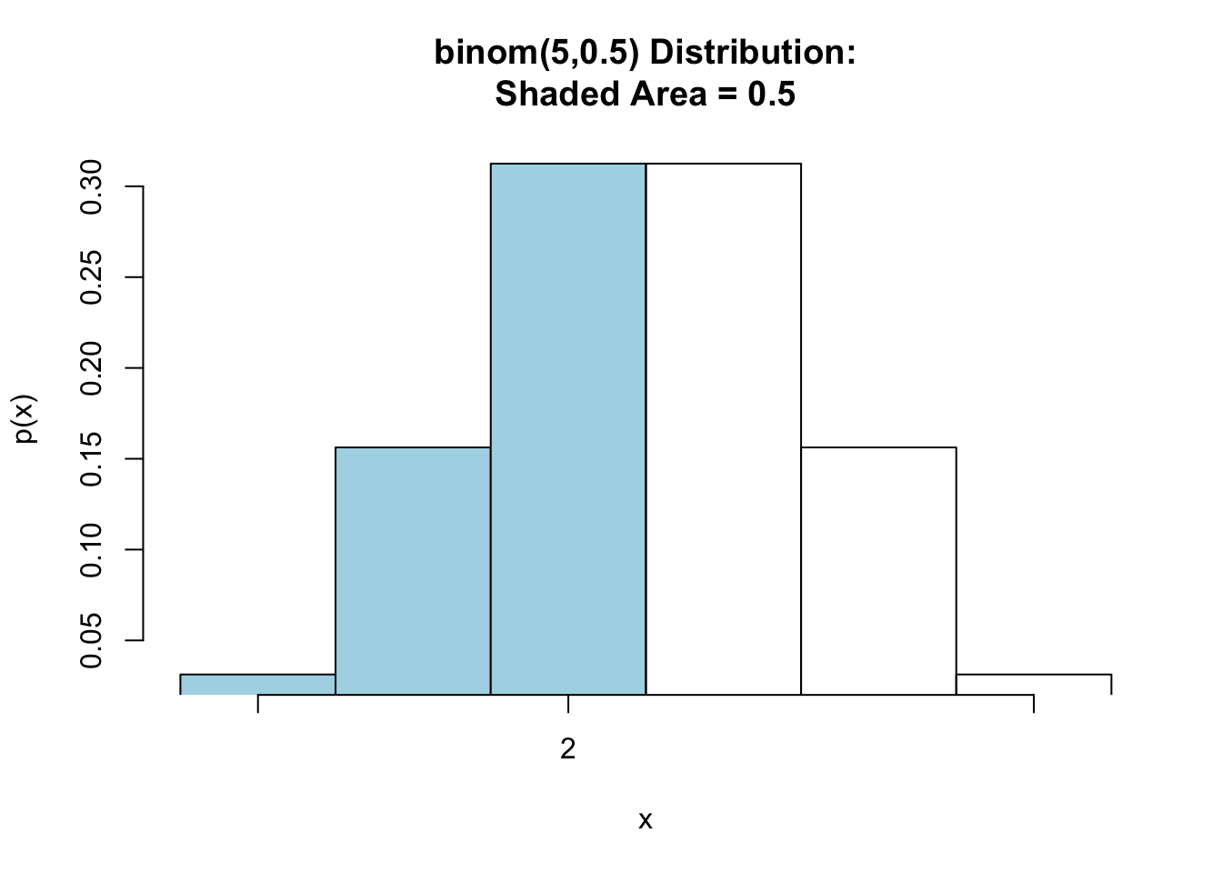

Figure 7.8: Binomial Less Than: Shaded region represents the probability that there are less than 3 heads are tossed in 5 tosses of a fair coin.

## [1] 0.5

Thus, $\mbox{P}(X\leq 3)=$ 0.8125.

7.4.6.5 P(X >= 2 and X <= 4)

Say we are interested in finding the probability of tossing at least 2 but not more than 4 heads in five tosses of a fair coin, $\mbox{P}(2\leq X\leq 4)$. Put another way, this is the probability of tossing 2, 3, or 4 heads in five tosses of a fair coin. See Figure [Binomial Between].

pbinomGC(c(2,4),region="between", size=5,prob=0.5,graph=TRUE)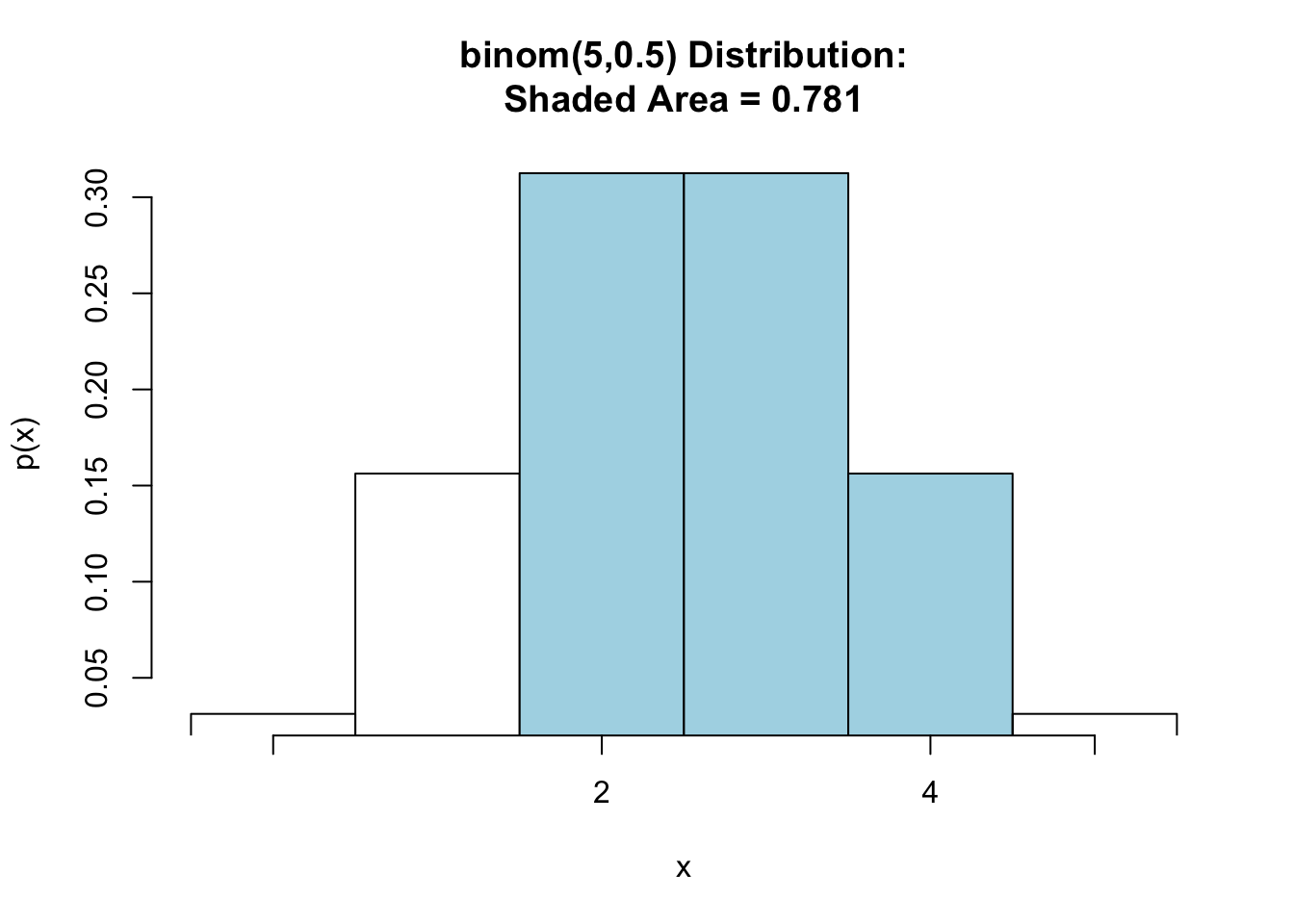

Figure 7.9: Binomial Between: Shaded region represents the probability that at least 2 but at most 4 heads are tossed in 5 tosses of a fair coin.

## [1] 0.78125

Thus, $\mbox{P}(1\leq X\leq 4)=$ 0.78125.

7.4.6.6 P(X = 2)

Finally, suppose we want to find the probability of tossing exactly 2 heads in five tosses of a fair coin. See Figure[Binomial Equal].

pbinomGC(c(2,2),region="between", size=5,prob=0.5,graph=TRUE)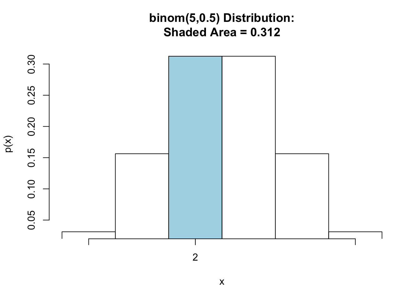

Figure 7.10: Binomial Equal: Shaded region represents the probability that exactly 2 heads are tossed in 5 tosses of a fair coin.

## [1] 0.3125

So, $\mbox{P}(X=2)=$ 0.3125.

7.4.6.7 Expected Value and Standard Deviation for a Binomial Random Variable

Although expected value and standard deviation can be calculated for binomial random variables the same way as we did before, there are nice formulas that make the calculation easier!

For a binomial random variable, $X$, based on $n$ independent trials with probability of success $p$,

the expected value is $EV(X)=n\cdot p$
the standard deviation is $SD(X)=\sqrt{n\cdot p\cdot (1-p)}$.

Example: Let’s compute the expected value for the random variable $X=\mbox{ number of heads tossed}$ in the five coin toss example.

The expected value, $EV(X)=5 \cdot 0.5 = 2.5$. Using R,

5*0.5

## [1] 2.5

The standard deviation, $SD(X) =\sqrt{5\cdot 0.5\cdot (1-0.5)}= 1.118034$. Using R,

sqrt(5*0.5*(1-0.5))

## [1] 1.118034

7.5 Continuous Random Variables

Continuous Random Variables: A continuous random variable is a random variable whose possible values come from a range of real numbers, with no smallest difference between values.

Example: If you let $X$ be the height in inches of a randomly selected person, then $X$ is a continuous random variables. That’s because there is no smallest possible difference between thow heights: two people could be an differ by one inch, 0.1 inches, 0.001 inches, and so on.

Non-Example: If you let $X$ be the number of shoes a randomly-selected person owns, then $X$ is not a continuous random variable. After all, there is a smallest difference between two values of $X$: one person can have two shoes and another could have three, but nobody can have any value in between, such as 2.3 shoes!

Note: For a discrete random variable, $X$, we could find the following types of probabilities:

$P(X=x)$
$P(X\leq x)$
$P(X < x)$
$P(X\geq x)$
$P(X>x)$
$P(a\leq X\leq x)$

For a continuous random variable, $X$, we can only find the following types of probabilities:

$P(X\leq x)$
$P(X < x)$
$P(X\geq x)$
$P(X>x)$
$P(a\leq X\leq x)$

In other words, we were able to find the probability that a discrete random variable took on an exact value. We can only find the probablity that a continuous random variable falls in some range of values. Since we cannot find the probability that a continuous random variable equals an exact value, the following probabilities are the same for continuous random variables:

$P(X\leq x)=P(X < x)$
$P(X\geq x)=P(X>x)$
$P(a \leq X \leq x)=P(a < X < b)=P(a \leq X < b)=P(a < X\leq b)$

7.5.1 Probability Density Functions for Continuous Random Variables

For discrete random variables, we used the probability distribution function (pdf) to find probabilities. The pdf for a discrete random variable was a table or a histogram.

For continuous random variables, we will use the probability density function (pdf) to find probabilities. The pdf for a continous random variable is a smooth curve.

The best way to get an idea of how this works is to examine an example of a continous random variable.

7.5.2 A Special Continuous Random Variable: Normal Random Variable

The only special type of continuous random variable that we will be looking at in this class is a normal random variable. There are many other continuous random variables, but normal random variables are the most commonly used continuous random variable.

A normal random variable, $X$

is said to have a normal distribution,

is completely characterized by it’s mean, $EV(X)=\mu$, and it’s standard deviation, $SD(X)=\sigma$, (These are the symbols that were introduced in Chapter 5.)

has a probability density function (pdf) that is bell-shaped, or symmetric. The pdf is called a normal curve. An example of this curve is shown in Figure[Normal Curve].

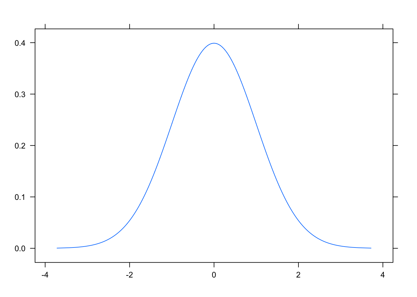
Figure 7.11: Normal Curve

Here is an important special type of normal random variable:

Standard Normal Random Variable: A normal random variables with mean, $\mu=0$, and standard deviation, $\sigma=1$ is called a standard normal random variable.

The following is a list of features of a normal curve.

Centered at the mean, $\mu$. Since it is bell-shaped, the curve is symmetric about the mean.
$P(X\leq \mu)=0.5$. Likewise, $P(X\geq \mu)=0.5$.
Normal Random Variables follow the 68-95 Rule (also called the Empirical Rule)
- The probability that a random variable is within one standard deviation of the mean is about 68%. This can be written: \[P(\mu-\sigma< X < \mu+\sigma)\approx 0.68\]
- The probability that a random variable is within two standard deviations of the mean is about 95%. This can be written: \[P(\mu-2\sigma< X < \mu+2\sigma)\approx 0.95\]
- The probability that a random variable is within three standard deviations of the mean is about 99.7%. This can be written: \[P(\mu-3\sigma< X < \mu+3\sigma)\approx 0.997\]

Example: Suppose that the distribution of the heights of college males follow a normal distribution with mean $\mu=72$ inches and standard deviation $\sigma=3.1$ inches. Let the random variable $X=\mbox{heights of college males}$. We can approximate various probabilities using the 68-95 Rule.

About 95% of males are between what two heights?
P(________ < $X$ < ________) $\approx$ 0.95

Answer: We can determine this using the second statement of the 68-95 Rule. The two heights we are looking for are:

72-2*3.1

## [1] 65.8

72+2*3.1

## [1] 78.2

So, P(65.8 < $X$ < 78.2) $\approx$ 0.95. See Figure[68-95 Rule Between 65.8 and 78.2].

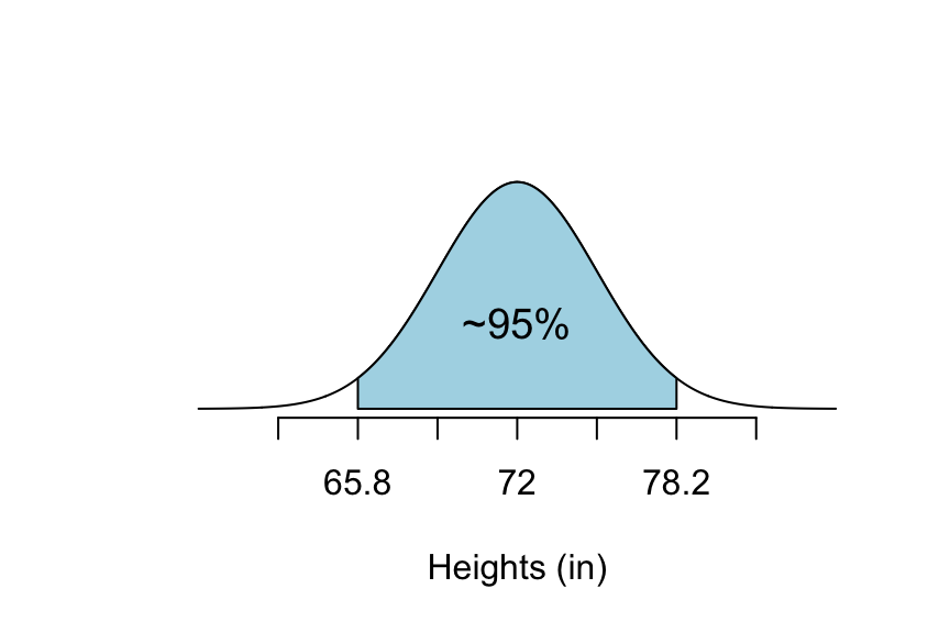
68-95 Rule Between 65.8 and 78.2: The shaded part of this graph is the percentage of college males that are between 65.8 inches and 78.2 inches tall.

Figure 7.12: 68-95 Rule Between 65.8 and 78.2: The shaded part of this graph is the percentage of college males that are between 65.8 inches and 78.2 inches tall.

About what percentage of males are less than 65.8 inches tall?
P($X$ < 65.8) $\approx$ _________

Answer: We know that 65.8 is two standard deviations below the mean. We also know that about 95% of males are between 65.8 and 78.2 inches tall. This means that about 5% of males are either shorter than 65.8 inches or taller than 78.2 inches. Since a normal curve is symmetric, then 2.5% of males are shorter than 65.8 inches and 2.5% of males are taller than 78.2 inches.

So, P($X$ < 65.8) $\approx$ 2.5%. See Figure[68-95 Rule Below 65.8].

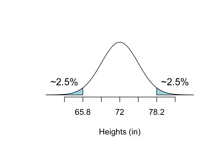
Figure 7.13: 68-95 Rule Below 65.8: The shaded part of this graph is the percentage of college males that are shorter than 65.8 inches.

About what percentage of males are more than 65.8 inches tall? P($X$ > 65.8) $\approx$ _____________

Answer: Since about 2.5% of males are shorter than 65.8 inches, then 100%-2.5%=97.5% of males are taller than 65.8 inches.

So, P($X$ > 65.8) $\approx$ 97.5%. See Figure [68-95 Rule Above 65.8].

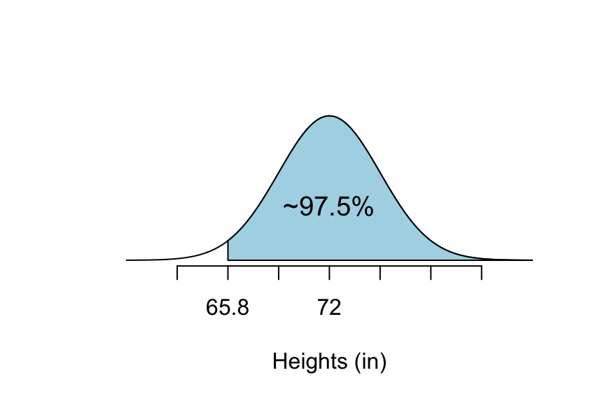
Figure 7.14: 68-95 Rule Above 65.8: The shaded part of this graph is the percentage of college males that are taller than 65.8 inches.

We can see the 68-95 Rule in action using the following app. You may find this app useful for various problems throughout the semester. All you have to do is change the mean and standard deviation to match the problem you are working on.

require(manipulate)
EmpRuleGC(mean=72,sd=3.1, xlab="Heights (inches)")

There is a function in R, similar to the one we used for binomial probability, that we can us to calculate probabilities other than those that are apparent from the 68-95 Rule. The pnormGC function will do this for you.

P$(X>70.9)$ can be found using the following code. See Figure[Normal Greater Than].

pnormGC(70.9,region="above", mean=72,sd=3.1, graph=TRUE)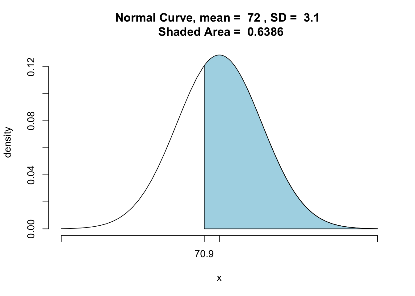

Figure 7.15: Normal Greater Than: The area of the shaded region is the percentage of males that are taller than 70.9 inches.

## [1] 0.6386448

Thus, P$(X>70.9)=$ 0.6386448.

P$(X< 69.4 \mbox{ or } X>79.1)$ can be found using the following code. See Figure[Normal Outside].

pnormGC(c(69.4,79.1),region="outside", mean=72,sd=3.1,graph=TRUE)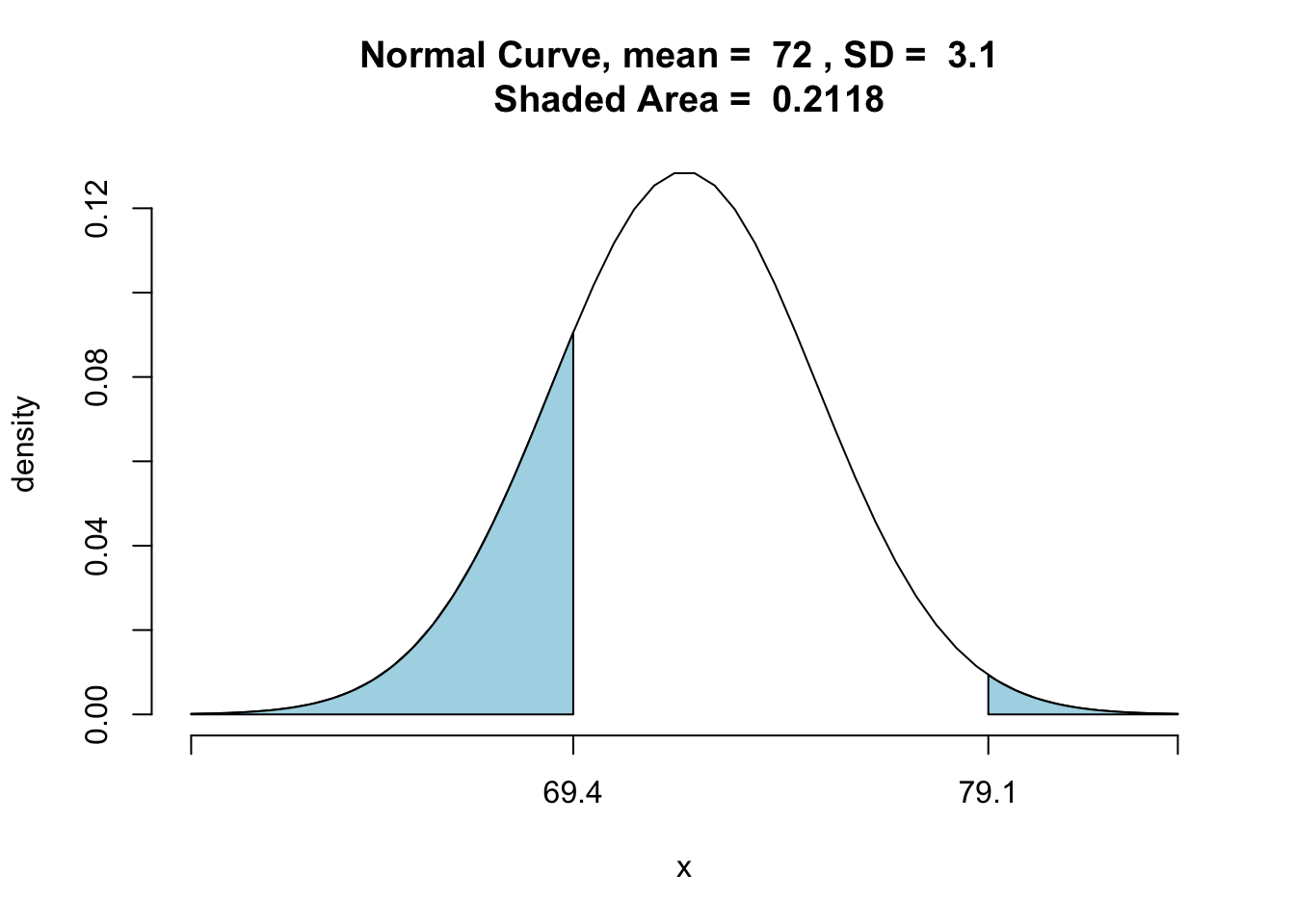

Figure 7.16: Normal Outside: The area of the shaded region is the percentage of males that are shorter than 69.4 inches or taller than 79.1 inches.

## [1] 0.2118174

Let’s switch this up a little. Suppose we want to know the height of a male that is taller than 80% of college men. Now we know the probability (or quantile) and we would like to know the $x$ that goes with it. Here, $x$ is called a percentile ranking. We are looking for $P(X\leq x)=0.80$.

This can be found using the qnorm function. This function requires three inputs - quantile, mean, and standard deviation. It returns the percentile ranking.

qnorm(0.80,mean=72,sd=3.1)

## [1] 74.60903

So, $x=74.6$. In other words, a male that is 74.6 inches tall is taller than about 80% of college men: P$(X<\leq 74.6)=$ 80%. We can use this number to look at the graph. See Figure[Quantile].

pnormGC(74.60903,mean=72,sd=3.1,region="below",graph=TRUE)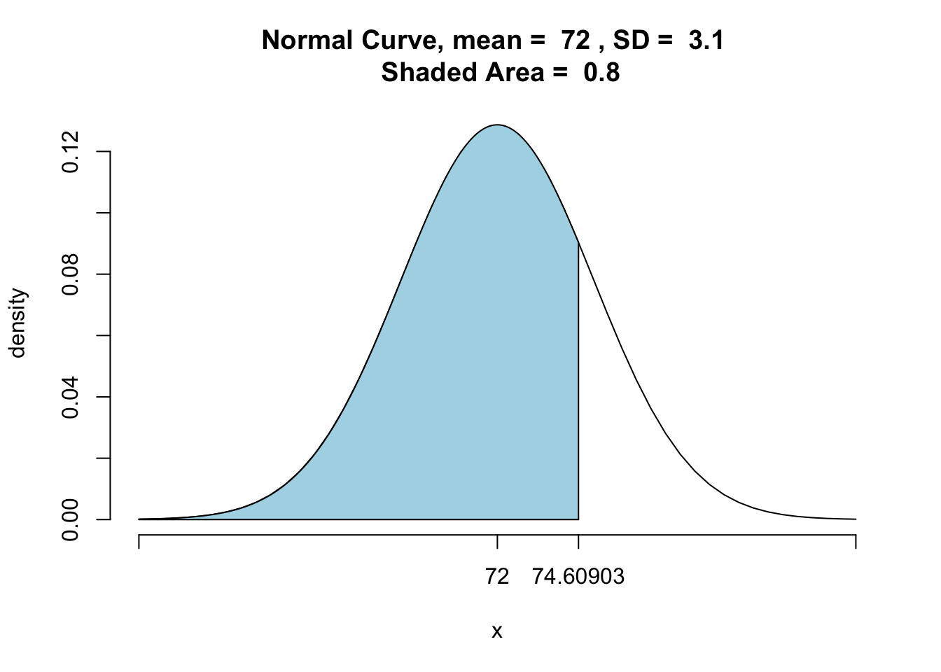

Figure 7.17: Quantile: This graph represents the 80th quantile.

## [1] 0.8000004

7.6 Approximating Binomial Probabilities

Recall that a binomial random variable is defined by the number of trials, $n$, and the probability of success, $p$. If the number of trials, $n$, is large enough, a binomial random variable can be well approximated by a normal distribution on two conditions:

There are at least 10 successes, $n\cdot p \geq 10$.
There are at least 10 failures, $n \cdot (1-p) \geq 10$.

This can be seen by looking at the graphs of a binomial random variable. You can see that as $n$ increases, the binomial distribution begins to look more and more like the normal curve using the following app.

require(manipulate)
BinomNorm()

You can also use the following app to see that if either the expected number of successes is too small ($n\cdot p \leq 10$) or the expected number of failures is too small ($n \cdot (1-p) \leq 10$), the normal curve does not do a very good job at approximating the binomial distribution.

require(manipulate)
BinomSkew()

7.7 Thoughts on R

7.7.1 New R Functions

Know how to use these functions:

pbinomGC
pnormGC
qnorm

Elementary Statistics with R