Notes for Instructors

First Models

We introduce classification trees with the tree::tree() function, using only the default control-values at first. Thus:

library(tigerstats)
help(m111survey)  # a familiar "stock-example" data frame for our students
trMod <- tree(sex ~ ., data = m111survey)
plot(trMod); text(trMod)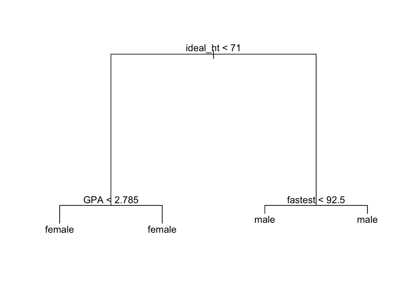

The interactive app treeDetective() helps students connect graphs such as the above with the tree model as a predictive device. It is also useful in showing students how the a tree model deals with missing values.

The construction of a simple classification tree based on two numerical predictor variables can easily be shown in a series of slides.

Understanding Output

We find it very helpful to spend some time on the concept of deviance, so that students can understand all parts of the text-based view of the model:

trMod

## node), split, n, deviance, yval, (yprob)
##       * denotes terminal node
## 
## 1) root 68 93.320 female ( 0.55882 0.44118 )  
##   2) ideal_ht < 71 39 15.780 female ( 0.94872 0.05128 )  
##     4) GPA < 2.785 6  7.638 female ( 0.66667 0.33333 ) *
##     5) GPA > 2.785 33  0.000 female ( 1.00000 0.00000 ) *
##   3) ideal_ht > 71 29  8.700 male ( 0.03448 0.96552 )  
##     6) fastest < 92.5 5  5.004 male ( 0.20000 0.80000 ) *
##     7) fastest > 92.5 24  0.000 male ( 0.00000 1.00000 ) *

This also helps students understand the output of:

summary(trMod)

## 
## Classification tree:
## tree(formula = sex ~ ., data = m111survey)
## Variables actually used in tree construction:
## [1] "ideal_ht" "GPA"      "fastest" 
## Number of terminal nodes:  4 
## Residual mean deviance:  0.1975 = 12.64 / 64 
## Misclassification error rate: 0.04412 = 3 / 68

Tree-Control

Next we bring in the idea that one can grow trees of various “sizes.” We introduce the tree::tree.control() function and carefully explain all of its arguments.

By this point we will have introduced regression trees, too.

Train/Quiz/Test

When students are accustomed to making trees of various sizes and interpreting them, we move on to the basic ideas of predictive modeling, especially the notion of training vs. test sets. Quiz sets are introduced early, in order to deal with the common case in which one builds a number of models and compares them on a quiz set in order to choose the “best” one. The Shiny app tuneTree() is useful for this purpose. The app permits students construct to new trees “by hand”, adjusting tree.control() parameters as they like, and keeps a record of all the trees they have made. Here students will encounter for the first time the U-shaped graphs of performance vs. size and get the idea that models of “intermediate” size tend to perform best on new data.

Pruning Trees

Cross-validation is somewhat beyond the scope of our elementary classes, so when it comes to standard procedures for making and assessing many tree models, we prefer tree::prune.tree(). This procedures works backwards from a relatively “large” initial tree, systematically snipping off nodes to produce successively smaller sub-trees whose performance on a quiz set is assessed. Students can use a plot of the results to choose a favorite model for evaluation on the test set, just as they might have used the graph in tunetree() to select a “best” tree.